Beyond the Visible
Reinterpreting Dark Matter and Dark Energy as Projected Curvature from a Sixty‑Dimensional Gravitational Bulk

Summary

The sixty dimensional framework proposes that the dark sector, which accounts for ninety five percent of the universe’s gravitational influence, is not made of unseen matter or exotic energy. Instead, it is the projection of curvature that resides in a sixty dimensional gravitational bulk. In this view, the familiar four dimensional Einstein equations describe only the small fraction of bulk curvature that reaches our observable spatial dimensions, while the remaining higher dimensional geometry appears as dark matter and dark energy. Humans cannot perceive these dimensions because of sensory, neural, and geometric limits. Metric gradient interferometry and AI based high dimensional inference provide the first empirical pathway for detecting the residual tidal fields that arise from the bulk. This paradigm reframes the dark sector as a geometric shadow of a much larger spacetime and marks the beginning of a transition from a limited three dimensional perspective to dimensional agency, which is the capacity to detect and interpret the higher dimensional curvature that shapes the observable universe.

The Case for a Higher-Dimensional Universe

Modern cosmology rests on a striking imbalance: only about five percent of the universe’s energy–mass content is made of ordinary baryonic matter, while the remaining ninety‑five percent is attributed to dark matter and dark energy. These 'dark' components have never been directly detected; they are inferred solely from their gravitational influence on cosmic structure and expansion. Their physical nature remains unknown, making the “dark sector” not a physical explanation but a placeholder for whatever geometry or physics is missing from current theory.

The framework used to describe this composition is the ΛCDM model, the standard model of cosmology. It assumes a universe governed by general relativity, filled with ordinary matter, cold dark matter (CDM), and a cosmological constant (Λ) representing dark energy. Within this model, baryonic matter—the familiar atomic matter of stars, planets, gas, and dust—accounts for only about five percent of the total. The remaining mass–energy is assigned to two hypothetical components: dark matter (≈27%), a non‑luminous mass introduced to explain galaxy rotation curves, cluster dynamics, and gravitational lensing; and dark energy (≈68%), a smooth, negative‑pressure field invoked to account for the accelerating expansion of the universe.

These precise fractions arise because they are the only values that allow ΛCDM to match all major cosmological observations simultaneously:

  • The cosmic microwave background fixes both the baryon density and the total matter density through the pattern of its acoustic peaks
  • Baryon acoustic oscillations constrain the expansion scale
  • Large‑scale structure measurements determine how quickly matter can clump under gravity
  • Type Ia supernovae reveal the recent acceleration of cosmic expansion

When these independent datasets are fitted together, only one composition satisfies all constraints: roughly five percent baryonic matter, twenty‑seven percent dark matter, and sixty‑eight percent dark energy. Any other mixture fails to reproduce at least one of these observational pillars.

The fact that ninety‑five percent of the universe is assigned to undetected components raises a deeper question: are dark matter and dark energy real substances, or signs that our geometric description of gravity is incomplete? The standard ΛCDM model assumes that gravity is computed strictly within a four‑dimensional spacetime—three spatial dimensions plus time. But General Relativity itself does not require this specific dimensionality. If the underlying geometry has additional spatial dimensions, then the gravitational effects currently attributed to the dark sector could instead arise from how higher‑dimensional curvature appears when projected onto our observable four‑dimensional slice.

Annex A provides detailed explanations and symbol definitions for all equations included throughout the text of the manuscript.

General Relativity provides a geometric description of gravity, in which the Einstein field equations relate the curvature of spacetime to the energy–momentum tensor. In four dimensions, the Einstein equations take the form

$$ G_{\mu\nu} = 8\pi G_4 T_{\mu\nu} $$

where Gμν is the Einstein tensor and Tμν is the stress–energy tensor of matter and radiation. Although this formulation is usually written for a 3+1‑dimensional spacetime, the mathematics of General Relativity places no restriction on the number of dimensions. The Einstein equations can be generalised to an arbitrary number of spatial dimensions, and higher‑dimensional extensions have been explored in Kaluza–Klein theory, string theory, and braneworld models (Overduin and Wesson 1997; Maartens and Koyama 2010). These frameworks show that higher‑dimensional curvature can generate effective four‑dimensional gravitational phenomena that mimic the presence of additional matter or energy.

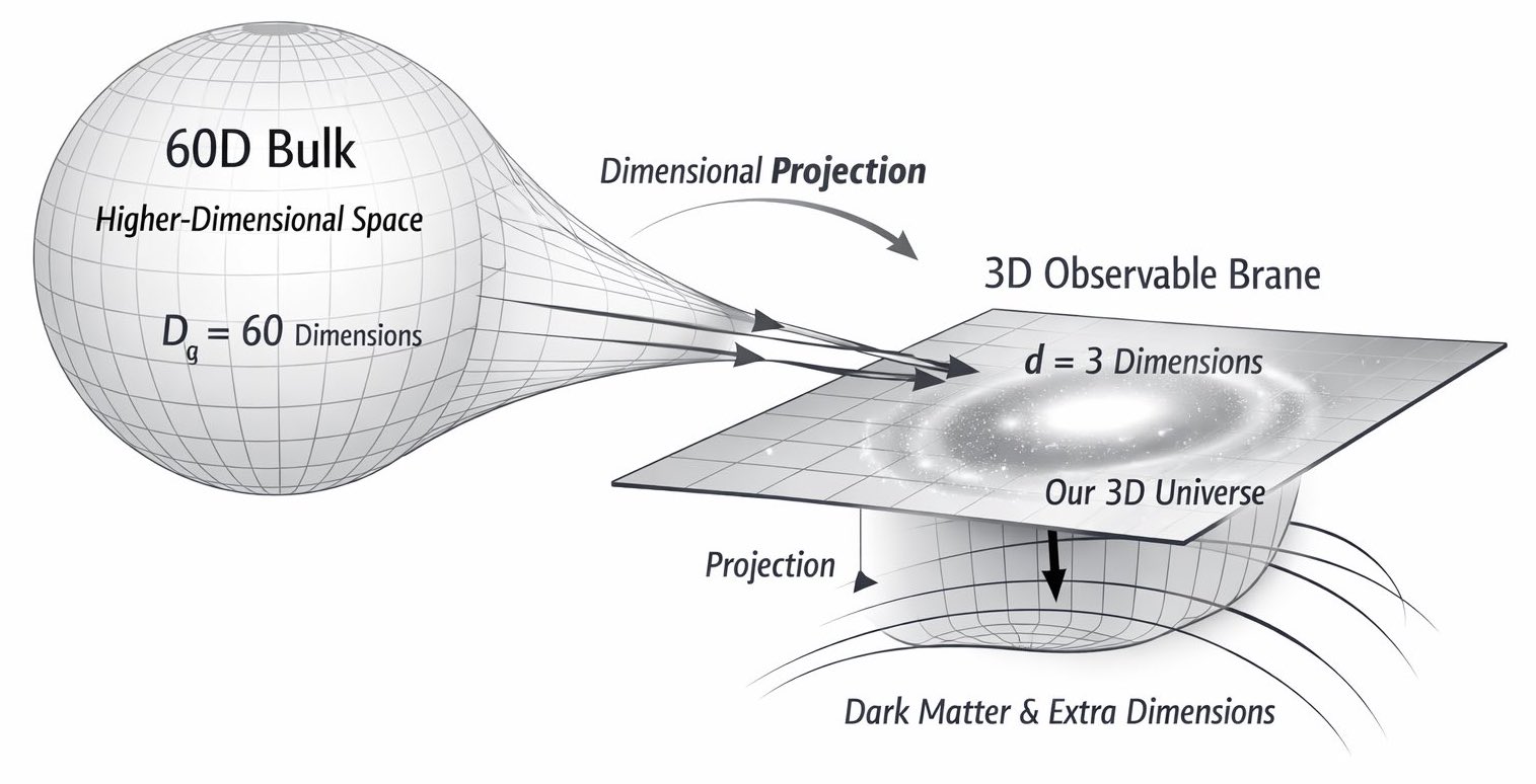
The central hypothesis of this work is that the dark sector is not composed of unseen substances, but instead arises from the projection of curvature in a higher‑dimensional gravitational bulk onto our (3+1)-dimensional spacetime. If gravity propagates through Dg spatial dimensions while we directly experience only three, then most of the total curvature generated by the full geometry would lie outside our observable manifold. Only the portion of curvature that projects into the three spatial dimensions we inhabit would appear to us as “ordinary” matter and energy.

Observationally, only about five percent of the universe’s total gravitational influence behaves as baryonic matter. This fraction provides a direct empirical clue to the dimensional structure of the gravitational field. If the visible fraction corresponds to the ratio of observable spatial dimensions to the total number of gravity‑active dimensions, then

$$ \frac{3}{D_g} \approx 0.05 $$

which yields

$$ D_g \approx 60 $$

This relation is not a speculative numerology but an observational dimensional constraint. The same ratio that defines the visible fraction of gravitational influence defines the proportion of curvature accessible to three spatial dimensions. In effect, the universe itself encodes its dimensional architecture in the relative strength of the dark and visible sectors. The inference Dg ≈ 60 therefore arises directly from cosmological data: the observed 5 %–95 % split between baryonic and dark components is treated not as a composition problem but as a projection ratio within the geometry of spacetime.

Unlike dimensional counts imposed by theoretical considerations, this inference is empirically grounded. The remaining ninety‑five percent of gravitational curvature resides in additional spatial directions that couple only weakly to the observable slice. Under this interpretation, Dg ≈ 60 is not a free parameter but a measurable property of the gravitational bulk—an observationally motivated constraint on the effective dimensionality of spacetime itself.

This framework differs fundamentally from existing higher‑dimensional theories. In string theory, the number of dimensions is fixed by mathematical consistency; in braneworld models, extra dimensions are introduced to modify gravity at specific scales; and in Kaluza–Klein theory, additional dimensions are compactified to unobservable sizes. In all such approaches, dimensionality is a theoretical input. In contrast, the dimensional‑projection framework treats the number of gravity‑active spatial dimensions as an observable quantity, constrained directly by the measured ratio between visible and dark gravitational influence. Rather than postulating extra dimensions for mathematical elegance or unification, it infers them from the universe’s curvature budget. This inversion of logic — deriving dimensionality from cosmological data rather than imposing it — makes the framework empirically anchored and testable, linking the dark‑sector fraction to the underlying geometry of spacetime.

The implications of this hypothesis are significant. If the dark sector reflects higher‑dimensional curvature rather than unseen forms of matter or energy, then the universe is embedded in a far richer geometric structure than the four‑dimensional picture suggests. In such a scenario, the effective Einstein equations governing gravity in our observable spacetime would necessarily contain additional terms arising from how curvature in the higher‑dimensional bulk projects onto our three‑dimensional spatial slice. This is structurally similar to braneworld models, where bulk effects appear through the projected Weyl tensor Eμν (Shiromizu et al. 2000), but here these terms acquire a different interpretation: they represent the portion of bulk curvature that does not fully project into the observable manifold. Within this framework, the gravitational phenomena currently attributed to dark matter and dark energy emerge naturally as the four‑dimensional imprint of curvature residing in the higher‑dimensional bulk.

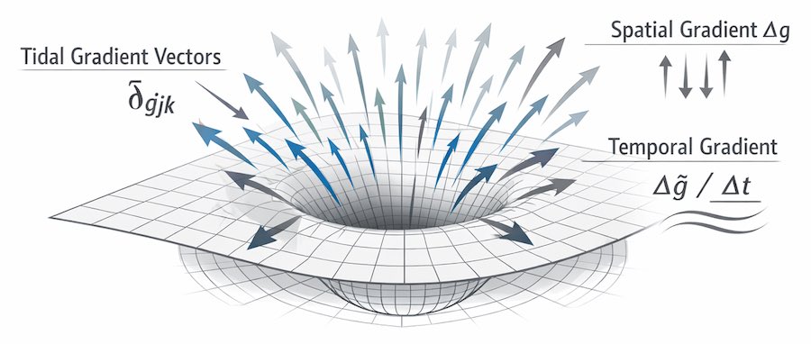
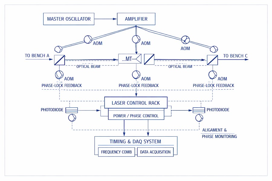
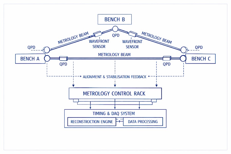
A major obstacle in evaluating this hypothesis is that no existing instrument can measure the kind of gravitational information required to detect higher‑dimensional curvature. Current gravitational‑wave interferometers, such as LIGO and Virgo, measure integrated strain along long, one‑dimensional baselines. This makes them exquisitely sensitive to the overall stretching and squeezing of spacetime along a path, but completely insensitive to how the metric varies from point to point in space. In other words, they measure global distortions, not the local tidal gradients that would reveal geometric structure beyond four dimensions.
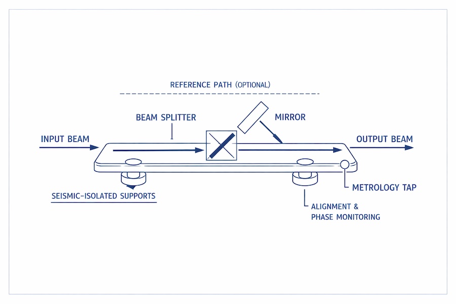
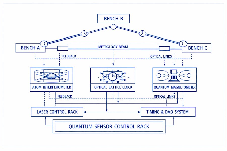
The type of measurement required does not yet exist. To test the hypothesis, one would need an instrument capable of mapping the spatial derivatives of the metric—the way spacetime curvature changes across a finite three‑dimensional region. This is the motivation for metric‑gradient interferometry, proposed in this work (see Sections 7, 8 and Annex C). Instead of measuring strain along a single arm, such an instrument would directly sample the local tidal field

\[ \partial_i g_{jk}, \]

which captures the gradient of the metric rather than its path‑averaged change. Ordinary interferometers smooth over these gradients, effectively erasing the small‑scale curvature structure that a higher‑dimensional geometry would imprint on spacetime.

A metric‑gradient interferometer would do something fundamentally different: it would measure spatial derivatives of the metric at multiple nearby points, allowing it to reconstruct the tidal‑gradient pattern within a finite volume. These gradients encode the local curvature texture of spacetime — the small‑scale anisotropies, directional dependencies, and cross‑component correlations that higher‑dimensional models predict.
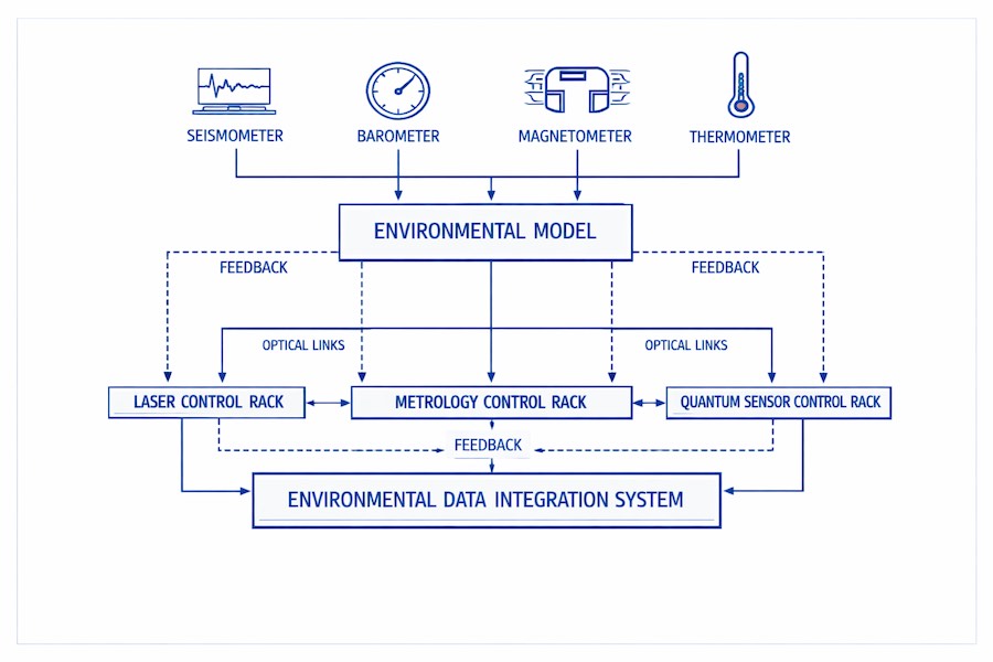
 By capturing these local variations, the instrument would access geometric information that current detectors cannot, opening a new observational window onto higher‑dimensional curvature.

Developing an instrument capable of measuring metric gradients would solve only half of the problem. Even if such a device could map the fine‑grained tidal structure of spacetime, the resulting data would be extraordinarily high‑dimensional and far beyond human intuitive comprehension. Detecting higher‑dimensional curvature therefore requires not only a new form of measurement, but also a new form of analysis—one capable of recognising geometric patterns that do not exist in ordinary four‑dimensional intuition.

Artificial intelligence plays a crucial role in this endeavour. Higher‑dimensional geometry cannot be visualised or mentally represented by humans, but AI systems can naturally encode and manipulate high‑dimensional manifolds. By training AI on metric‑gradient data, it becomes possible to infer the structure of the higher‑dimensional bulk from its projection onto the four‑dimensional brane. In this sense, AI becomes more than a computational tool: it functions as a scientific interface between human observers and the larger geometric structure of spacetime.

The case for a higher‑dimensional universe arises from the mismatch between the observed matter content of the cosmos and the gravitational phenomena it produces. By interpreting the dark sector as a projection effect of higher‑dimensional curvature—and by developing both the measurement techniques and computational tools required to detect such curvature—it becomes possible to test this idea empirically rather than philosophically. This approach reframes the dark sector as a geometric signal awaiting detection and defines a concrete experimental pathway for determining whether the gravitational structure of the universe extends beyond the four dimensions we directly observe. 
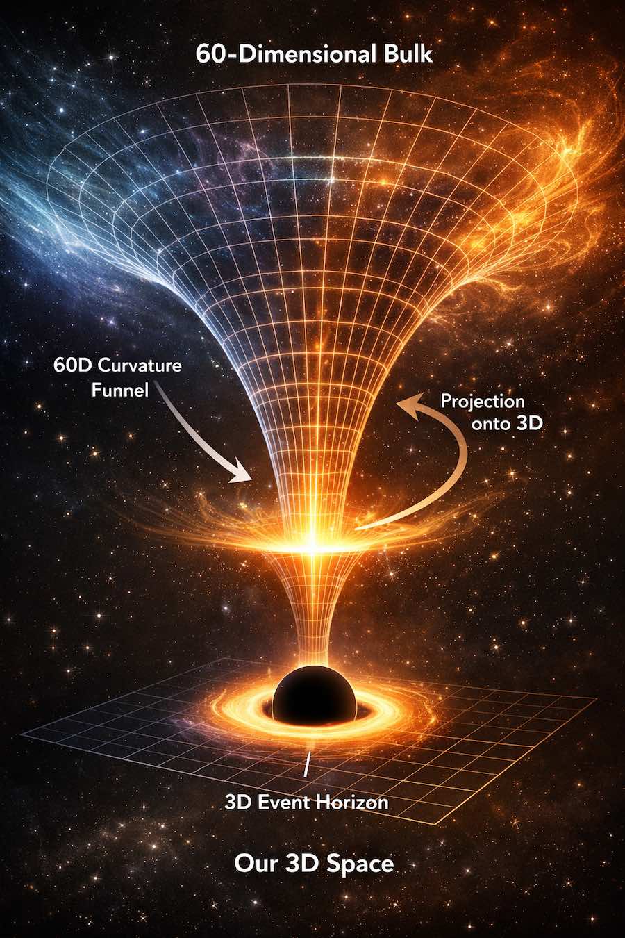
This framework therefore leads to a natural geometric interpretation: the observable universe behaves as a three‑dimensional projection of curvature originating in a much higher‑dimensional gravitational manifold, as depicted in the illustration below.

Image

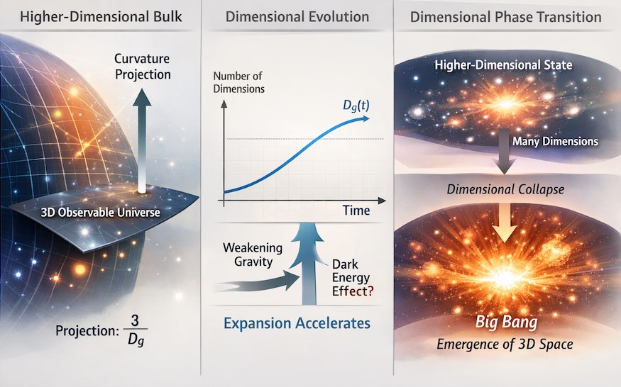
If the observable universe is a lower‑dimensional projection of a higher‑dimensional bulk, then the initial conditions traditionally attributed to the Big Bang may instead reflect geometric features of the higher‑dimensional manifold. The implications of this shift are developed in Section 4.

God geometrizes continually.

Plato

The Dimensional Projection Framework

The dimensional projection framework provides the mathematical foundation for the hypothesis introduced in Section 1. Its purpose is to formalise how a higher‑dimensional gravitational field GAB gives rise to the effective four‑dimensional curvature gμν observed in our universe. In this view, the dark sector is not a material component but the residual influence of curvature residing in spatial directions orthogonal to the observable manifold. When the full geometry is projected onto a (3+1)-dimensional hypersurface, part of the curvature is retained while the remainder is hidden, producing the apparent discrepancy between visible matter and total gravitational influence.

Higher‑Dimensional Einstein Equations

The starting point is the generalisation of the Einstein field equations to a bulk spacetime with Dg spatial dimensions and one temporal dimension:

$$ G_{AB} = 8\pi G_{D_g} T_{AB}, $$

where indices A, B span the full (Dg +1)-dimensional manifold. The bulk metric GAB contains curvature components both tangent to the observable hypersurface and extending into the additional (Dg -3) spatial dimensions. These extra components do not vanish; they simply do not appear directly in the induced four‑dimensional geometry.

When the bulk equations are projected onto a four‑dimensional hypersurface, the resulting effective Einstein equations acquire additional geometric terms. This structure is well established in braneworld models, where the effective equations take the form:

$$ G_{\mu\nu} = 8\pi G_4 T_{\mu\nu} + \mathcal{E}_{\mu\nu} + \mathcal{F}_{\mu\nu} $$

with Eμν representing the projected bulk Weyl tensor and Fμν containing quadratic corrections in the brane energy–momentum tensor (Shiromizu et al. 2000). In the dimensional projection framework, Eμν is interpreted as the geometric origin of the dark sector.

Projection Geometry and the Gauss–Codazzi Structure

The projection from the bulk to the observable universe is defined by the induced metric

$$ g_{\mu\nu} = G_{AB} \, e^A_{\ \mu} e^B_{\ \nu} $$

where eAμ are the tangent vectors to the hypersurface. The embedding of the hypersurface in the bulk is characterised by the extrinsic curvature

$$ K_{\mu\nu} = e^A_{\ \mu} e^B_{\ \nu} \nabla_A n_B $$

With nb the normal vector to the hypersurface.

The Gauss–Codazzi equations relate the intrinsic curvature of the hypersurface to the bulk curvature and the extrinsic curvature. These relations demonstrate that the effective four‑dimensional gravitational field necessarily contains contributions from higher‑dimensional geometry. In the dimensional projection framework, these extrinsic contributions are interpreted as the dark sector.

Inferring the Dimensionality of the Gravitational Bulk

As discussed in Section 1, only a small fraction of the universe’s gravitational influence—approximately five percent—projects into the observable three spatial dimensions. Interpreting this fraction as the ratio of visible to total curvature yields the dimensional‑projection law:

\[ D_g = \frac{3}{0.05} = 60 \]

This result implies that the majority of curvature resides in the remaining Dg -3 spatial dimensions. In effective four‑dimensional descriptions, this hidden curvature manifests as the gravitational phenomena currently attributed to dark matter and dark energy.

The Eleven‑Dimensional Dark‑Matter Subspace

The same projection logic can be applied to the dark‑matter component specifically. Dark matter accounts for approximately twenty‑seven percent of the universe’s gravitational influence. If this fraction corresponds to curvature projecting from a particular subspace of the higher‑dimensional bulk, then

$$ \frac{3}{D_{\mathrm{DM}}} \approx 0.27 $$

which yields an eleven‑dimensional dark‑matter submanifold embedded within the full sixty‑dimensional bulk. The coincidence between this value and the dimensionality of M‑theory is notable, but the present framework does not rely on supersymmetry, compactification, or string‑theoretic constraints. Instead, the dimensionality emerges directly from cosmological observations, offering a novel empirical interpretation of the eleven‑dimensional structure that appears in theoretical physics.

Information Loss and the Origin of the Dark Sector

The information loss inherent in the projection process explains why higher‑dimensional curvature appears as additional gravitational influence rather than as observable matter. When a higher‑dimensional object is projected onto a lower‑dimensional manifold, geometric features such as curvature, topology, and connectivity may be compressed or obscured. This phenomenon is familiar in lower‑dimensional analogues: a three‑dimensional object projected onto a two‑dimensional plane loses information about its depth, and a four‑dimensional object projected onto three dimensions would lose information about its higher‑dimensional structure (Coxeter, 1963). The dimensional projection framework extends this intuition to the sixty‑dimensional bulk, interpreting the dark sector as the shadow of higher‑dimensional curvature.

Geometric Interpretation of Dark Matter and Dark Energy

The framework also provides a natural explanation for the smoothness and universality of the dark sector. If dark matter and dark energy arise from higher‑dimensional curvature, then their distribution is determined by the geometry of the bulk rather than by local particle interactions. This explains why dark matter appears collisionless and why dark energy exhibits a uniform density across the observable universe. It also suggests that the large‑scale structure of the cosmos is influenced by the geometry of the higher‑dimensional bulk, providing a geometric interpretation of cosmic acceleration and the formation of the cosmic web.

To summarise the structure developed in this section, the combination of higher‑dimensional Einstein equations, projection geometry, and observationally inferred dimensionality defines a coherent and unified reinterpretation of the dark sector. For clarity in what follows, this framework will be referred to as Dimensional‑Projection Gravity (DPG): a theory in which the gravitational phenomena attributed to dark matter and dark energy arise from the projection of curvature in a sixty‑dimensional bulk onto the observable (3+1)-dimensional manifold. DPG provides a geometric, non‑material explanation for the dark sector and establishes the foundation for the dynamical and cosmological implications explored in subsequent sections.

Gravity and Curvature in a 60-Dimensional Bulk

The hypothesis that gravity propagates in a sixty‑dimensional spatial manifold requires a re‑examination of the geometric structure of spacetime and the behaviour of curvature in higher dimensions. In General Relativity, the gravitational field is encoded in the curvature of a four‑dimensional Lorentzian manifold, and the Einstein field equations relate this curvature to the energy–momentum tensor. When the dimensionality of spacetime is increased, the mathematical structure of the theory changes in ways that have direct physical consequences. The strength of gravity, the propagation of curvature, and the form of the gravitational potential all depend on the number of spatial dimensions. This section develops the geometric and physical implications of a sixty‑dimensional bulk and explains how such a structure can reproduce the observed gravitational phenomena in our three‑dimensional slice.

The starting point is the generalisation of the Einstein–Hilbert action to Dg spatial dimensions. The action takes the form

$$ S = \frac{1}{16\pi G_{D_g}} \int d^{D_g+1}x \, \sqrt{-G} \, R $$

Varying this action with respect to the metric yields the higher‑dimensional Einstein equations,

$$ G_{AB} = 8\pi G_{D_g} T_{AB} $$

These equations describe how matter and energy curve the sixty‑dimensional bulk. The gravitational constant GDg has different dimensions than the four‑dimensional Newtonian constant G4, and the relationship between them depends on the geometry of the extra dimensions (Overduin and Wesson, 1997).

Gravitational Potential in Higher Dimensions

One of the most important consequences of higher‑dimensional gravity is the modification of the gravitational potential. In Dg spatial dimensions, the Newtonian potential generated by a point mass M scales as

$$ \Phi(r) \propto \frac{1}{r^{D_g - 2}} $$

For Dg = 3, this reduces to the familiar inverse‑square law. For Dg = 60, the potential falls off as 1/r58, which would render gravity effectively unobservable at macroscopic scales unless the extra dimensions are compactified, warped, or otherwise geometrically suppressed. This is consistent with the idea that the majority of curvature resides in the higher‑dimensional bulk and does not project strongly into our observable three‑dimensional slice. The effective four‑dimensional gravitational potential is therefore not the fundamental potential of the bulk, but a projection of it.

Gauss–Codazzi Structure and Extrinsic Geometry

The projection process can be understood using the Gauss–Codazzi formalism. When a four‑dimensional hypersurface is embedded in a higher‑dimensional manifold, its intrinsic curvature is related to the bulk curvature and the extrinsic curvature of the embedding. The Gauss equation takes the form

$$ R_{\mu\nu\alpha\beta} = G_{ABCD} \, e^A_{\ \mu} e^B_{\ \nu} e^C_{\ \alpha} e^D_{\ \beta} + K_{\mu\alpha} K_{\nu\beta} - K_{\mu\beta} K_{\nu\alpha} $$

where GABCD is the higher‑dimensional Riemann tensor and Kμν is the extrinsic curvature. The Codazzi equation relates derivatives of the extrinsic curvature to components of the bulk curvature. These relations demonstrate that the effective four‑dimensional curvature contains contributions from both intrinsic and extrinsic geometric quantities. In the dimensional projection framework, the extrinsic contributions are interpreted as the dark sector.

Projected Bulk Weyl Tensor and the Dark Sector

The projected bulk Weyl tensor,

$$ \mathcal{E}_{\mu\nu} = G_{ABCD} \, n^A n^C e^B_{\ \mu} e^D_{\ \nu} $$

plays a central role in this interpretation. In braneworld models, Eμν encodes the influence of the bulk geometry on the brane and can mimic the effects of dark matter and dark energy (Maartens and Koyama, 2010). In the present framework, Eμν arises from the curvature of the sixty‑dimensional bulk and accounts for the observed gravitational phenomena that cannot be explained by visible matter. The dimensional projection law,

$$ \frac{3}{D_g} = 0.05 $$

implies that only five percent of the bulk curvature projects into the observable three‑dimensional manifold. The remaining ninety‑five percent appears as the dark sector.

Curvature Degrees of Freedom in Sixty Dimensions

The structure of curvature in a sixty‑dimensional bulk is qualitatively different from that in four dimensions. The Riemann tensor in Dg spatial dimensions has

$$ N_R = \frac{D_g^2 (D_g^2 - 1)}{12} $$

independent components. For Dg = 3, this yields twenty components; for Dg = 60, it yields over ten million. This enormous increase in geometric degrees of freedom provides a natural reservoir for the dark sector. The effective four‑dimensional curvature is a low‑dimensional projection of a vastly richer geometric structure. The complexity of the bulk curvature also suggests that higher‑dimensional gravitational phenomena may exhibit patterns or correlations that are not captured by four‑dimensional models.

Gravitational Wave Propagation and Bulk Leakage

The propagation of gravitational waves is also modified in higher dimensions. In four dimensions, gravitational waves have two polarisation states and propagate at the speed of light. In Dg spatial dimensions, the number of polarisation states increases, and the propagation of curvature can occur in directions orthogonal to the brane. This leakage of gravitational energy into the bulk can weaken the amplitude of gravitational waves observed in four dimensions, providing a potential observational signature of higher‑dimensional gravity (Cardoso et al. 2003). The absence of such signatures in current gravitational‑wave data suggests that the extra dimensions must be geometrically suppressed, consistent with the projection framework.

Black Holes as Curvature Funnels in the Bulk

In the Dimensional‑Projection Gravity framework, a black hole is interpreted not as a singularity in four dimensions but as the visible intersection of a deep curvature funnel extending into the sixty‑dimensional bulk. The familiar Schwarzschild or Kerr geometry arises only after projection onto our three‑dimensional spatial slice. The full curvature structure is governed by the higher‑dimensional Einstein equations, and in vacuum regions of the bulk, TAB = 0, so the geometry is determined entirely by the higher‑dimensional curvature tensor RABCD .

The projection of this bulk curvature onto the observable manifold is governed by the Gauss equation, and near a black hole the extrinsic curvature becomes large and rapidly varying, reflecting the steep gradient of the bulk curvature funnel. The apparent singularity of a four‑dimensional black hole corresponds to the limit in which the projection map from the bulk to the brane becomes non‑invertible:

\[ \det\!\left( \frac{\partial x^\mu}{\partial X^A} \right) = 0 \]

The higher‑dimensional curvature funnel can be characterised by the behaviour of the bulk Kretschmann scalar,

\[ K_{60} = R_{ABCD} R^{ABCD} \]

which remains finite throughout the bulk but grows sharply along the funnel axis. The projected four‑dimensional Kretschmann scalar,

\[ K_{4} = R_{\mu\nu\alpha\beta} R^{\mu\nu\alpha\beta} \]

inherits this growth through the Gauss relation, giving rise to the familiar divergence at r = 0 in the Schwarzschild solution. In DPG, this divergence is not fundamental but arises from the compression of a large region of bulk curvature into a point-like projection.

The gravitational potential associated with a bulk curvature funnel also differs from the four‑dimensional case. In sixty spatial dimensions, the Newtonian potential of a localised mass‑energy distribution scales as

\[ \Phi_{60}(r) \propto \frac{1}{r^{58}} \]

but the projection onto the brane yields an effective potential

\[ \Phi_{4}(r) = \Pi(\Phi_{60}) \propto \frac{1}{r} \]

with corrections arising from the extrinsic curvature and the projected Weyl tensor. These corrections modify the near‑horizon geometry and may produce observable deviations in black‑hole shadow asymmetry, photon‑ring thickness, and polarisation structure.

In this interpretation, black holes are not isolated anomalies but localised intersections of the same higher‑dimensional curvature that gives rise to the dark sector. Dark matter corresponds to weak, distributed projections of bulk curvature, while black holes correspond to strong, localised projections. Both phenomena arise from the same geometric mechanism, differing only in intensity and localisation.

The illustration below provides a visual representation of the curvature funnel, showing how a deep sixty‑dimensional structure projects into our three‑dimensional manifold as a black hole.

visual representation of the curvature funnel, showing how a deep sixty‑dimensional structure projects into our three‑dimensional manifold as a black hole

Bulk Geometry and Large Scale Structure

The geometry of the sixty‑dimensional bulk also influences the large‑scale structure of the universe. If dark matter arises from curvature in an eleven‑dimensional subspace of the bulk, as suggested by the relation

$$ \frac{3}{D_{\mathrm{DM}}} = 0.27 $$

then the distribution of dark matter is determined by the geometry of this subspace. This provides a geometric interpretation of the observed properties of dark matter, including its collisionless behaviour and its role in structure formation. Similarly, if dark energy arises from curvature in the remaining forty‑nine dimensions, then cosmic acceleration may be a geometric effect rather than a manifestation of a cosmological constant.

Summary

The behaviour of gravity and curvature in a sixty‑dimensional bulk provides a natural explanation for the dark sector. The effective four‑dimensional gravitational field is a projection of a much larger geometric structure, and the majority of curvature resides in dimensions orthogonal to our own. This framework unifies the dark matter and dark energy phenomena as manifestations of higher‑dimensional curvature and shows that black holes are localised intersections of the same projection mechanism, appearing as the three‑dimensional cross‑sections of deep curvature funnels in the bulk. Together, these elements provide a geometric foundation for the development of metric‑gradient interferometry and AI‑based higher‑dimensional inference. Taken as a whole, they constitute the core of Dimensional‑Projection Gravity.

Dimensional Evolution and Its Cosmological Implications

Within the broader framework of Dimensional‑Projection Gravity, the evolution of the gravitational dimensionality Dg (t) becomes a central driver of cosmological behaviour. DPG treats the observable universe as a dynamically evolving projection of curvature from a sixty dimensional bulk, and the time dependence of this projection determines how much of the bulk curvature appears in four dimensions.

In this framework, time is not a coordinate of the sixty dimensional gravitational bulk. The bulk is a purely geometric structure: timeless, static, and defined only by its curvature relationships. The apparent evolution arises entirely on the four dimensional hypersurface, where the projection of bulk curvature changes as Dg (t) evolves.

Time appears only when a four dimensional hypersurface is projected from the bulk. The projection induces a metric signature, a causal structure, and an ordering of events that we interpret as temporal flow. What evolves is not the bulk itself, but the position and orientation of the four dimensional slice as it moves through the higher dimensional curvature.

Dark matter corresponds to the static component of this projection, while dark energy reflects the time dependent way in which the four dimensional hypersurface intersects the deeper geometry. In this sense, time is not a fundamental dimension of reality but a property of the projection itself.

This perspective aligns with the deeper insight that geometry, matter, and the appearance of time are inseparable aspects of a single structure, an idea captured succinctly by Einstein:

Time and space and gravitation have no separate existence from matter.

Einstein

A natural extension of the dimensional‑projection framework is to consider the possibility that the number of gravity‑active dimensions, Dg , is not fixed but evolves over cosmic time. If higher‑dimensional curvature projects into our three‑dimensional slice according to the ratio 3/Dg , then any time‑dependence in Dg (t) directly alters the effective energy density and expansion dynamics observed in four dimensions. This leads to a modified Friedmann equation of the form

\[ H^2 = \frac{8\pi G}{3}\rho_{\text{eff}}(t) + \Delta_{\text{dim}}(t) \]

where Δdim (t) arises from the time derivative of the projection factor,

\[ \frac{d}{dt}\!\left(\frac{3}{D_g(t)}\right) \]

and acts as an additional contribution to the cosmic expansion rate. In this picture, the universe accelerates not because of a cosmological constant but because the projection of curvature into three dimensions becomes progressively diluted as Dg (t) increases. This provides a geometric mechanism for dark‑energy‑like behaviour without invoking vacuum energy or exotic fields.

Dimensional growth therefore offers a compelling reinterpretation of cosmic acceleration: as the number of gravity‑active dimensions increases, the fraction of curvature that projects into our observable manifold decreases, weakening the effective gravitational pull and producing a repulsive term in the expansion dynamics. This mechanism parallels aspects of braneworld acceleration and dynamical compactification models, but arises here from a simple geometric principle rather than from specific field‑theoretic constructions.

Allowing Dg to vary also reshapes the interpretation of the early universe. In standard cosmology, the Big Bang corresponds to a singular state of diverging density and curvature. In a dimensional‑evolution framework, this singularity can be replaced by a dimensional phase transition in which a high‑dimensional gravitational system begins projecting into a lower‑dimensional manifold. The emergence of three large spatial dimensions becomes a dynamical event rather than an initial condition, and the Big Bang marks the onset of stable projection rather than the origin of spacetime itself. This perspective aligns with ideas from string‑gas cosmology and braneworld collision models, but provides a more direct geometric interpretation: the early universe may have possessed many more active dimensions, with only three becoming macroscopically accessible as the projection stabilised.

Taken together, these considerations suggest that cosmic expansion, dark‑energy‑like acceleration, and even the Big Bang itself may be understood as consequences of evolving dimensionality within a higher‑dimensional gravitational bulk. The dimensional‑projection framework therefore offers a unified geometric interpretation of several outstanding cosmological phenomena, grounded in the behaviour of curvature across a dynamically evolving higher‑dimensional space.

In this sense, the cosmological consequences of evolving dimensionality arise naturally within Dimensional‑Projection Gravity, which provides a unified geometric account of dark matter, dark energy, and the large‑scale evolution of the universe.

Dimensional Evolution and Curvature Projection

Image

Description: This figure above illustrates the conceptual structure of the dimensional‑projection framework and its cosmological implications. The left panel depicts the higher‑dimensional gravitational bulk with Dg spatial dimensions, represented as a large ambient space containing curvature distributed across many directions. The observable universe is shown as a three‑dimensional submanifold embedded within this bulk. Only a fraction of the total curvature projects into this submanifold, with the projection factor given by 3/Dg .

The central panel shows the time evolution of the dimensionality, Dg (t). As the number of gravity‑active dimensions increases, the projection factor decreases, reducing the amount of curvature that appears within the observable three‑dimensional slice. This dilution of projected curvature generates an effective repulsive contribution to the expansion rate, producing dark‑energy‑like behaviour without invoking a cosmological constant.

The right panel illustrates the dimensional phase transition interpretation of the Big Bang. Instead of a singular origin, the early universe is shown as a high‑dimensional state in which curvature is distributed across many spatial directions. The emergence of three large spatial dimensions corresponds to the stabilisation of the projection onto the observable manifold. This transition replaces the classical singularity with a geometric event in which the effective dimensionality of the universe changes.

Together, the panels convey how evolving dimensionality modifies the Friedmann dynamics, produces late‑time acceleration, and reframes the Big Bang as a transition in the structure of the higher‑dimensional gravitational bulk.

Annex B provides further detailed information on dimensional evolution and the modified Friedmann equation.

Why We Cannot Perceive the Extra Dimensions

Human perceptual limitations take on a precise meaning within Dimensional‑Projection Gravity. If the observable universe is a projection of curvature from a sixty‑dimensional bulk, then our sensory and cognitive systems—evolved entirely within a three‑dimensional manifold—are structurally incapable of accessing or representing the additional dimensions. The invisibility of the higher‑dimensional bulk is therefore not accidental but an inevitable consequence of the projection process itself.

The inability of humans to perceive the additional spatial dimensions posited by the sixty‑dimensional bulk is not a biological accident but a geometric inevitability. Perception is constrained by the structure of the sensory apparatus, the neural architecture that processes sensory data, and the dimensionality of the manifold in which these systems evolved. Human cognition is adapted to a three‑dimensional environment, and the brain constructs a model of the world based on two‑dimensional retinal input that is reconstructed into a three‑dimensional perceptual space. This reconstruction process is highly optimised for the ecological demands of terrestrial life but is fundamentally incapable of representing higher‑dimensional geometry. The extra dimensions are therefore not merely unseen—they are unrepresentable within the human perceptual and cognitive framework.

The first reason for this limitation is sensory. Human sensory organs are embedded in a three‑dimensional spatial manifold and can only detect variations in fields that project onto this manifold. The retina, for example, is a two‑dimensional surface that receives electromagnetic radiation and reconstructs a three‑dimensional world through depth cues such as occlusion, motion parallax, and stereopsis (Palmer, 1999). If a four‑dimensional object were to intersect our three‑dimensional space, the retina would only receive a three‑dimensional slice of that object. The same logic applies to higher‑dimensional curvature: the sensory apparatus can only detect the projection of the higher‑dimensional metric onto the observable manifold. The majority of curvature in the sixty‑dimensional bulk does not project strongly into the three spatial dimensions accessible to human senses and therefore remains imperceptible.

The second reason is neural. The human brain constructs a model of the world using neural representations that are intrinsically low‑dimensional. The visual cortex, for example, encodes features such as edges, motion, and depth using hierarchical representations that ultimately converge on a three‑dimensional model of the environment (Hubel and Wiesel, 1962). These representations are not arbitrary; they are shaped by evolutionary pressures that favoured organisms capable of navigating a three‑dimensional world. The brain has no mechanism for representing or manipulating higher‑dimensional geometric structures. Even mathematical reasoning about higher dimensions relies on symbolic manipulation rather than perceptual intuition. This cognitive limitation is not a matter of training or experience but a structural constraint of the neural architecture.

The third reason is geometric. When a higher‑dimensional object is projected onto a lower‑dimensional manifold, information is inevitably lost. This is a consequence of the fact that projection is not an invertible operation: multiple higher‑dimensional configurations can produce the same lower‑dimensional projection. A familiar example is the projection of a three‑dimensional object onto a two‑dimensional plane. The resulting silhouette contains no information about the object’s depth or internal structure. Similarly, a four‑dimensional object projected onto three dimensions loses information about its higher‑dimensional geometry (Coxeter, 1963). In the sixty‑dimensional bulk, this information loss is extreme. The effective four‑dimensional metric is a low‑dimensional shadow of a vastly richer geometric structure, and the human perceptual system has no access to the lost dimensions.

The fourth reason is dynamical. The Einstein field equations in four dimensions describe how matter and energy curve spacetime, but they do not account for curvature in dimensions orthogonal to the observable manifold. The effective four‑dimensional Einstein equations contain additional terms arising from the projection of the bulk geometry, such as the projected Weyl tensor Eμν (Shiromizu et al. 2000). These terms influence the motion of matter and the propagation of light, but they do so in ways that mimic the presence of additional matter or energy rather than revealing the existence of extra dimensions. The dark sector is therefore a perceptual illusion: a higher‑dimensional geometric effect that appears, from the perspective of a three‑dimensional observer, as an unexplained gravitational influence.

The fifth reason is evolutionary. Human sensory and cognitive systems evolved under selective pressures that favored survival in a three‑dimensional environment. There was no evolutionary advantage to perceiving higher‑dimensional curvature, as such curvature does not manifest directly in the three‑dimensional world. The brain therefore evolved to ignore or compress any information that does not fit within its three‑dimensional model of reality. This evolutionary constraint is analogous to the way in which the human ear is sensitive to a limited range of frequencies or the way in which the human eye is sensitive to a limited range of wavelengths. Perception is not a faithful representation of reality but an adaptive interface optimized for survival (Hoffman, 2019).

The sixth reason is mathematical. The number of independent components of the Riemann curvature tensor increases extremely rapidly as the number of spatial dimensions grows. In three spatial dimensions, the tensor has only twenty independent components, but in sixty dimensions the number exceeds ten million. This explosive growth in complexity means that the full curvature structure of a sixty‑dimensional bulk is far beyond what the human brain can intuitively represent or manipulate. Even in four dimensions, physicists rely heavily on symmetries, approximations, and computational tools to work with the Riemann tensor. The geometric richness of a sixty‑dimensional curvature field therefore lies far outside the representational capacity of biological cognition.

The final reason is epistemic. Human scientific understanding is grounded in models that can be visualised, verbalised, or mathematically formalised within the constraints of human cognition. Higher‑dimensional geometry cannot be visualised or intuitively understood, and its mathematical representation is too complex for direct human manipulation. Artificial intelligence, by contrast, can represent and manipulate high‑dimensional manifolds using distributed representations in neural networks. AI therefore becomes the first system capable of interfacing with the higher‑dimensional bulk, not because it has superior perception, but because it is not constrained by the representational limitations of biological cognition.

These perceptual, neural, geometric, and evolutionary constraints explain why the higher‑dimensional curvature central to DPG remains inaccessible to direct human experience, and why any empirical access to the sixty‑dimensional bulk must rely on instruments and AI‑based inference rather than biological perception.

From Todays Physics to a 60D-Aware Paradigm

The transition to a sixty‑dimensional understanding of gravity can be formalised within Dimensional‑Projection Gravity, the framework in which the observable universe is interpreted as a lower‑dimensional projection of curvature from a sixty‑dimensional bulk. DPG does not replace General Relativity; rather, it extends it by recognising that the four‑dimensional metric describes only the portion of curvature that projects into the observable manifold.

The transition from contemporary four‑dimensional physics to a framework that incorporates a sixty‑dimensional gravitational bulk represents a conceptual shift comparable to the transition from Newtonian mechanics to General Relativity. It requires reinterpreting the dark sector, revising the structure of the Einstein field equations, and expanding the mathematical and experimental tools used to study spacetime. This section outlines the pathway from the current paradigm to a 60D‑aware gravitational theory, emphasising continuity with established physics while highlighting the novel insights enabled by the dimensional projection framework.

The starting point is the recognition that the dark sector is not a failure of General Relativity but a failure of dimensional assumptions. General Relativity accurately describes how curvature influences the motion of matter and the propagation of light within a four‑dimensional manifold. Its success in predicting gravitational lensing, perihelion precession, gravitational redshift, and gravitational waves demonstrates the robustness of the theory (Will, 2014). The problem arises not from the equations themselves but from the assumption that the metric gμν captures the full curvature of spacetime. If gravity propagates in a sixty‑dimensional bulk, then the four‑dimensional metric is merely the induced metric on a lower‑dimensional hypersurface, and the Einstein equations must be supplemented by additional terms arising from the projection of the bulk geometry.

This reinterpretation aligns with the structure of higher‑dimensional theories already present in the literature. In Kaluza–Klein theory, the five‑dimensional metric produces both gravity and electromagnetism when projected onto four dimensions (Overduin and Wesson, 1997). In braneworld models, the effective four‑dimensional Einstein equations contain additional terms arising from the extrinsic curvature and the projected bulk Weyl tensor (Shiromizu et al. 2000). In string theory and M‑theory, the geometry of compact extra dimensions influences the effective four‑dimensional physics (Becker et al. 2007). The dimensional projection framework extends these ideas by deriving the number of gravity‑active dimensions from cosmological observations rather than from mathematical constraints.

The next step is to reinterpret the dark sector in geometric terms. The observed matter fraction of approximately five percent suggests that only a small portion of the bulk curvature projects into the observable three‑dimensional manifold. The dimensional projection law, as previously described, implies that gravity propagates in sixty spatial dimensions. The remaining fifty‑seven dimensions contribute to the effective four‑dimensional curvature through the projected Weyl tensor Eμν , which appears in the effective Einstein equations as an additional gravitational source. This provides a geometric interpretation of dark matter and dark energy: they are not substances but manifestations of higher‑dimensional curvature.

This interpretation resolves several long‑standing puzzles in cosmology. The collisionless behaviour of dark matter, its role in structure formation, and its apparent lack of electromagnetic interactions follow naturally from its geometric origin. Similarly, the uniform density of dark energy and its role in cosmic acceleration can be understood as a projection of curvature in dimensions orthogonal to the observable manifold. The dimensional projection framework therefore unifies the dark matter and dark energy phenomena as different manifestations of the same higher‑dimensional structure.

The transition to a 60D‑aware paradigm also requires revising the mathematical tools used to describe spacetime. The Riemann tensor in sixty spatial dimensions has over ten million independent components, far beyond the representational capacity of traditional analytical methods. This necessitates the use of computational tools, particularly artificial intelligence, to represent and manipulate high‑dimensional curvature fields. AI systems can operate in latent spaces with hundreds or thousands of dimensions, making them uniquely suited to modelling the geometry of the sixty‑dimensional bulk. This marks a shift from human‑centred mathematical intuition to machine‑assisted geometric inference.

Experimentally, the transition requires instruments capable of detecting the influence of higher‑dimensional curvature. Conventional gravitational‑wave detectors measure integrated strain along one‑dimensional baselines and are therefore insensitive to the spatial derivatives of the metric that encode higher‑dimensional effects. Metric‑gradient interferometry addresses this limitation by measuring the local tidal field, ∂igjk, in a finite region of space. By reconstructing the metric‑gradient tensor and subtracting known four‑dimensional sources, it becomes possible to isolate residual curvature attributable to the higher‑dimensional bulk. This provides the first empirical pathway for testing the dimensional projection framework.

The transition also has implications for the interpretation of cosmological data. Observations of galaxy rotation curves, gravitational lensing, cosmic microwave background anisotropies, and large‑scale structure formation must be reinterpreted in terms of higher‑dimensional curvature. This does not invalidate existing data; rather, it provides a new geometric context for understanding it. For example, the apparent need for cold dark matter in structure formation may reflect the influence of curvature in the higher‑dimensional subspace associated with the dark matter fraction. Similarly, the accelerated expansion of the universe may reflect curvature in the remaining forty‑nine dimensions.

Finally, the transition to a 60D‑aware paradigm represents a philosophical shift in the understanding of spacetime. The assumption that the observable universe is representative of the whole is replaced by the recognition that the observable universe is a projection of a much larger geometric structure. This shift parallels earlier transitions in the history of physics, such as the move from geocentrism to heliocentrism and from absolute space to curved spacetime. In each case, expanding the dimensional framework led to deeper insights into the structure of the universe. The dimensional projection framework continues this tradition by extending the reach of empirical science into the higher‑dimensional bulk.

Geometry is the key to unlocking the deepest secrets of the universe.

Roger Penrose

Within this extended theoretical framework, Dimensional‑Projection Gravity provides the conceptual and mathematical foundation for a 60D‑aware paradigm, unifying the dark sector, higher‑dimensional curvature, and the empirical tools needed to explore the remaining 95% of gravitational reality.

Metric‑Gradient Interferometry: Concept and Role

Within the framework of Dimensional‑Projection Gravity, metric‑gradient interferometry (MGI) serves as the first experimental methodology capable of probing the higher‑dimensional curvature that does not project into the observable four‑dimensional metric. Whereas conventional detectors measure only integrated strain, MGI is designed to detect the local spatial variation of the metric—precisely the quantity that carries information about curvature residing in the additional fifty‑seven gravity‑active dimensions.

The central claim of this framework is that if gravity propagates in more than three spatial dimensions, then the dominant part of spacetime curvature never appears as ordinary matter or radiation in our three‑dimensional slice. Conventional instruments—telescopes, particle detectors, and even gravitational‑wave interferometers—are therefore structurally incapable of detecting most of the geometry of the universe. Metric‑gradient interferometry is introduced as the first class of instrument explicitly designed to probe that hidden geometry by measuring not only changes in the metric, but spatial gradients of the metric itself.

In General Relativity, the spacetime metric gμν encodes the full gravitational field, and curvature is described by derivatives of the metric, ultimately forming the Riemann tensor Rρσμν (Einstein 1916; Misner et al. 1973). Conventional gravitational‑wave detectors such as LIGO, Virgo, and KAGRA operate in the weak‑field, linearised regime, where the metric is written as a flat Minkowski background plus a small perturbation (Maggiore 2008). These detectors are sensitive to the perturbation field, which manifests as differential changes in arm lengths and is observed as a dimensionless strain integrated along the interferometer arms.

However, if gravity propagates in a higher‑dimensional bulk with Dg gravity‑active dimensions, the effective four‑dimensional metric we observe is a projection of a higher‑dimensional bulk metric GAB , where indices A,B run over the full bulk and μ, ν label our four‑dimensional slice (Overduin & Wesson 1997; Maartens & Koyama 2010). In such scenarios, the higher‑dimensional Einstein equations project onto effective four‑dimensional equations containing additional geometric terms arising from the extrinsic curvature and the projected bulk Weyl tensor. These extra terms can mimic dark matter and dark energy in the effective four‑dimensional theory (Arkani‑Hamed 1998).

A strain‑based interferometer is sensitive only to the integrated effect of the perturbation field along its arms, but it is not designed to reconstruct spatial gradients of the metric in a local neighbourhood. In a higher‑dimensional context, the most informative quantity is not the perturbation itself, but its spatial variation—the metric‑gradient tensor ∂αgμν . This gradient encodes how curvature changes over space and is directly related to tidal fields and geodesic deviation. In four dimensions, the relative acceleration of nearby geodesics is governed by the geodesic deviation equation (Wald 1984), which relates the separation vector between neighbouring geodesics to the curvature tensor. A metric‑gradient interferometer is, in essence, an instrument optimised to reconstruct the local tidal field—i.e., the spatial variation of the metric—rather than only the integrated strain along a single baseline.

The conceptual shift is therefore from “strain interferometry” to “metric‑gradient interferometry.” In strain interferometry, one measures the difference in phase accumulated along two arms of length L, which is sensitive to a passing gravitational wave with wavelength much larger than the arm length. In metric‑gradient interferometry, one arranges multiple baselines with different orientations and separations, and uses their combined outputs to reconstruct the local tensor field describing spatial variations of the metric within a finite region. This requires not only multiple interferometric arms, but also careful control of environmental noise and auxiliary sensors to disentangle gravitational effects from local disturbances.

The role of higher dimensions enters through the effective four‑dimensional Einstein equations. In braneworld and Kaluza–Klein‑type models, the effective four‑dimensional Einstein tensor receives corrections from the bulk geometry, including contributions from the projected Weyl tensor Eμν and terms quadratic in the brane energy–momentum tensor Fμν (Shiromizu et al. 2000; Maartens & Koyama 2010). The projected Weyl term behaves like an effective “dark” stress–energy component from the four‑dimensional point of view. If the bulk has many gravity‑active dimensions, the majority of curvature may reside in directions orthogonal to our brane, and only a small fraction projects into the observable four‑dimensional metric.

A metric‑gradient interferometer is designed to be sensitive to the residual curvature that remains after all known four‑dimensional sources have been modelled and subtracted. In practice, this means that the instrument must operate in a regime where local Newtonian gravity, seismic noise, atmospheric effects, and electromagnetic disturbances are carefully monitored and accounted for. The interferometer’s outputs are then used to reconstruct an effective local tidal tensor, and a foreground model based on known physics is subtracted. The remaining residual field is interpreted as a candidate signal for higher‑dimensional curvature or other non‑standard gravitational phenomena.

The expected signal classes for such an instrument can be divided conceptually into at least two broad categories. The first is a smooth, quasi‑static background curvature corresponding to the effective influence of higher‑dimensional geometry on galactic and cosmological scales. This would manifest as a slowly varying tidal field that cannot be accounted for by visible matter or standard dark‑matter distributions. The second is localised or transient curvature gradients that might arise from compact higher‑dimensional structures, topological defects, or other non‑standard sources. In both cases, the key point is that the instrument is not looking for oscillatory strains with specific polarisations, as in gravitational‑wave astronomy, but for persistent or slowly varying deviations in the local metric gradient that cannot be explained by four‑dimensional sources.

The conceptual role of metric‑gradient interferometry in a sixty‑dimensional framework is therefore twofold. First, it provides an operational definition of “higher‑dimensional curvature” in terms of measurable quantities in our four‑dimensional slice. Second, it offers a concrete experimental pathway to test whether the dark sector can be understood as a projection effect of higher‑dimensional gravity. If the residual metric‑gradient field reconstructed by such instruments correlates with cosmological structures, gravitational anomalies, or other independent observables, this would provide strong evidence that our effective four‑dimensional description is incomplete and that additional gravity‑active dimensions are physically relevant.

In contrast to purely theoretical arguments for extra dimensions, metric‑gradient interferometry is explicitly empirical. It does not assume a specific compactification scheme, string model, or detailed bulk geometry. Instead, it starts from the general observation that any deviation from four‑dimensional General Relativity must ultimately manifest as a modification of the local metric and its gradients. By designing instruments that are sensitive to these gradients at high precision, one can probe a wide class of higher‑dimensional and modified‑gravity models in a model‑agnostic way. This aligns with the broader trend in gravitational physics, where precision experiments—such as gravitational‑wave detection, atom interferometry, and clock comparisons—are increasingly used to test the foundations of General Relativity and search for new physics (Dimopoulos et al. 2008; Tino et al. 2020). In this context, metric‑gradient interferometry provides the first direct experimental pathway for testing the predictions of Dimensional‑Projection Gravity by isolating the residual curvature expected from a sixty‑dimensional gravitational bulk.

Metric-Gradient Interferometer—Design, Deployment & Scientific Use

The preceding section introduced the conceptual role of the Metric‑Gradient Interferometer, while this section highlights the engineering, deployment, and analytical workflow required to build an instrument capable of isolating higher‑dimensional curvature in practice.

Concept and Measurement Principle

A metric‑gradient interferometer (MGI) is built on a fundamentally different measurement philosophy from strain‑based gravitational‑wave detectors. Whereas instruments such as LIGO, Virgo, and KAGRA measure integrated strain along kilometre‑scale baselines, an MGI is designed to measure local spatial derivatives of the metric, the quantities that encode how curvature varies across a finite region of space. This distinction is not merely technical; it reflects a shift from detecting transient waves to mapping the structure of spacetime itself.

In a four‑dimensional universe, the metric gradient is determined by local mass–energy distributions. But in higher‑dimensional models, the gradient may also contain contributions from curvature residing in the bulk. These contributions manifest as subtle tidal distortions, slow drifts, or persistent anisotropies that cannot be explained by known four‑dimensional physics. The MGI therefore functions as a local curvature microscope, capable of detecting geometric structure that is invisible to strain‑based detectors.

The conceptual illustration of the curvature‑gradient field—tidal gradient vectors, spatial gradients, and temporal gradients—captures this idea. Each component represents a different way in which curvature can vary, and each may carry signatures of higher‑dimensional geometry. The MGI’s purpose is to measure these variations with sufficient precision to distinguish between conventional gravitational effects and those arising from extra‑dimensional curvature.

A Conceptual Illustration of the Curvature Gradient Field

Image

The diagram shows tidal gradient vectors (δḡjk), spatial gradients (Δg), and temporal gradients (Δĝ / Δt), representing how local curvature variations may encode higher‑dimensional signals.

Design Principles

1. Geometric Configuration

The geometry of an MGI is central to its function. A single baseline provides only one scalar observable, insufficient for reconstructing even a single component of the metric‑gradient tensor. To measure curvature gradients, the instrument must sample spacetime in multiple directions and at multiple points. This requires non‑collinear baselines, ideally arranged in triangular or square configurations.

A triangular configuration allows the instrument to probe curvature across an enclosed area, enabling sensitivity to directional gradients and providing natural closure relations for consistency checks. A square or rectangular configuration adds redundancy, improves sensitivity to anisotropic gradients, and allows for over‑constrained reconstruction of the gradient tensor. The geometry must be chosen to balance practical engineering constraints with the mathematical requirements of tensor reconstruction.

2. Optical System

The optical system is the heart of the MGI. Unlike strain‑based detectors, which rely on long optical paths to amplify tiny changes in arm length, the MGI relies on differential phase shifts between parallel baselines. These phase differences encode the spatial variation of the metric across the separation distance.

Achieving the required sensitivity demands lasers with exceptional frequency stability, optical paths with minimal thermal drift, and interferometric readout systems capable of resolving phase differences far below the shot‑noise limit. The design must also ensure that parallel baselines remain geometrically stable over long periods, as even nanometre‑scale drifts can mimic or obscure genuine curvature‑gradient signals.

3. Integration of Quantum Sensors

Quantum sensors extend the MGI’s capabilities by providing independent, high‑precision measurements of gravitational potential and curvature. Atom interferometers measure phase shifts accumulated by matter waves, offering sensitivity to gravitational gradients demonstrated in both laboratory and field settings (Dimopoulos et al. 2008; Tino et al. 2020). Optical lattice clocks detect gravitational redshifts corresponding to centimetre‑scale height differences (McGrew et al. 2018), making them powerful probes of local curvature.

Integrating these sensors with the optical interferometer creates a multichannel measurement system. Each sensor type responds differently to gravitational and environmental disturbances, allowing cross‑validation and improved discrimination between genuine curvature signals and noise. This integration is essential for reconstructing the metric‑gradient tensor with high fidelity.

4. Environmental Isolation

Environmental noise is the dominant limitation for terrestrial MGIs. Seismic vibrations, atmospheric pressure fluctuations, temperature gradients, and electromagnetic interference all induce phase shifts that can overwhelm the gravitational signal. Effective isolation requires a combination of passive and active systems: vibration‑isolated platforms, vacuum enclosures, thermal shielding, and electromagnetic shielding.

Equally important is the deployment of a dense array of environmental sensors. These sensors provide the data needed to construct a detailed foreground model of expected four‑dimensional curvature contributions. Without accurate modelling and subtraction of these effects, the MGI cannot reliably identify residual signals that may originate from higher‑dimensional geometry.

5. Readout and Data Acquisition

The readout system must synchronise data from multiple baselines and auxiliary sensors with high temporal precision. This requires stable timing systems, high‑bandwidth data acquisition, and real‑time calibration pipelines. Because the MGI is intended for long‑duration monitoring, the readout system must also support continuous operation over months or years, with robust data storage and error‑correction mechanisms.

6. Reconstruction Algorithm

Reconstructing the metric‑gradient tensor is an inverse problem that requires careful mathematical treatment. The instrument response matrix encodes the geometry of the baselines, and the reconstruction must account for noise, incomplete sampling, and potential nonlinearities. Regularisation techniques—Tikhonov, Bayesian, or maximum‑likelihood—are used to stabilise the inversion (Tarantola, 2005). The algorithm must also incorporate environmental data to distinguish between four‑dimensional and higher‑dimensional contributions.

Physical Components of the MGI

Annex C provides detailed descriptions and illustrations of each physical component of the Metric‑Gradient Interferometer.

1. Optical Benches and Beam Handling Infrastructure

The optical benches provide the rigid, thermally stable platform on which the interferometric geometry is built. They are typically fabricated from ultralow‑expansion materials such as Zerodur, silicon carbide, or crystalline silicon, chosen for their negligible thermal expansion coefficients and mechanical stability. The benches host the beam splitters, mirrors, Faraday isolators, phase modulators, and reference cavities that define the optical paths.

The benches incorporate fiducial markers for laser‑tracker alignment, optical taps for diagnostic monitoring, and embedded wavefront sensors for real‑time beam‑quality assessment. Their geometry is optimised to minimise path‑length asymmetries and to ensure that parallel baselines remain truly parallel over long durations.

2. Laser Systems and Frequency References

The laser system is the metrological heart of the MGI. It must deliver narrow‑linewidth, ultra‑stable light with coherence lengths exceeding the baseline separation. This typically requires lasers locked to high‑finesse reference cavities using Pound–Drever–Hall stabilisation. The cavities themselves are housed in thermally stabilised enclosures with sub‑millikelvin temperature control and vibration isolation.

Electro‑optic and acousto‑optic modulators provide phase and frequency control, enabling heterodyne readout and active noise suppression. Optical frequency combs synchronise multiple laser channels and link the optical system to the timing infrastructure. Redundant laser heads and automated lock‑recovery systems ensure continuous operation over months or years.

3. Baseline Metrology and Alignment Sensors

Because the MGI measures differential phase shifts between parallel baselines, precise knowledge of baseline geometry is essential. Laser‑ranging metrology systems continuously measure the separation and orientation of optical paths with nanometre‑scale precision. These systems use heterodyne interferometry, frequency‑stabilised reference beams, and multi‑axis alignment sensors.

Quadrant photodiodes detect angular drift, while wavefront sensors monitor beam curvature and pointing. Inertial reference units provide low‑frequency stability, and tiltmeters detect slow ground motion. All metrology channels feed into active alignment systems that correct geometric drift in real time, ensuring that baseline variations do not masquerade as curvature‑gradient signals.

4. Quantum Sensor Modules

Quantum sensors provide independent, high‑precision measurements of gravitational potential and curvature. Atom interferometers require ultra‑high‑vacuum chambers, magnetic shielding, laser‑cooling systems, and precise atomic launch mechanisms. Their sensitivity depends on long interrogation times, stable magnetic fields, and accurate control of atomic trajectories.

Optical lattice clocks require ultra‑stable optical cavities, cryogenic or thermally stabilised housings, and vibration isolation platforms. Their performance is limited by blackbody radiation shifts, magnetic‑field gradients, and laser‑frequency noise. Both types of quantum sensors are mounted on mechanically decoupled platforms to prevent cross‑coupling with the optical interferometer.

Synchronisation links tie the quantum‑sensor outputs to the optical channels, enabling multisensor fusion during reconstruction of the metric‑gradient tensor.

5. Environmental Sensor Array

The environmental sensor array provides the data required to model and subtract environmental foregrounds. Seismometers measure ground motion across a broad frequency range, while barometers track atmospheric pressure fluctuations that induce gravitational loading. Magnetometers detect geomagnetic variations and local electromagnetic interference.

Thermometers and humidity sensors monitor thermal gradients and air‑density variations. Accelerometers detect local vibrations, and tiltmeters measure slow ground deformation. The sensors are distributed across the facility, with high‑density placement near optical benches, along baselines, and around quantum‑sensor modules.

Their data streams feed into real‑time environmental modelling pipelines, enabling dynamic subtraction of environmental noise and improving the fidelity of residual curvature‑gradient signals.

6. Vacuum, Thermal, and Electromagnetic Isolation Systems

The optical paths and quantum‑sensor chambers are housed within vacuum systems that suppress air‑density fluctuations, acoustic noise, and refractive‑index variations. Vacuum levels of 10⁻⁶–10⁻⁹ mbar are typical, depending on the subsystem. Vacuum tubes are constructed from stainless steel or carbon‑fibre composites, with low‑outgassing materials used for internal components.

Thermal isolation is achieved through multilayer insulation, cryogenic cooling (where required), and active thermal control loops. Temperature stability at the micro‑kelvin level is necessary for reference cavities and optical lattice clocks. Electromagnetic shielding—using mu‑metal, conductive enclosures, and filtered power systems—reduces magnetic and RF interference that could affect both optical and quantum sensors.

7. Control, Actuation, and Stabilisation Systems

Active control systems maintain alignment, suppress drift, and stabilise the instrument. Piezoelectric actuators adjust mirror positions with nanometre precision, while thermal actuators compensate for slow expansion of structural components. Inertial control systems stabilise the optical benches against low‑frequency vibrations.

In space‑based MGIs, micro‑Newton thrusters and drag‑free control systems maintain spacecraft formation geometry. These systems use inertial sensors and laser‑ranging data to adjust spacecraft positions continuously, ensuring that geometric drift remains below the threshold at which it would contaminate curvature‑gradient measurements.

All control loops operate with high bandwidth and low latency, ensuring that corrections do not introduce additional noise into the measurement channels.

8. Data Acquisition, Timing, and Synchronisation Infrastructure

The MGI requires high‑bandwidth data acquisition systems capable of synchronising optical, quantum, and environmental channels with sub‑nanosecond precision. Ultra‑stable clocks—often based on optical frequency standards—provide the timing reference. Timing distribution networks use fibre‑optic links, frequency combs, and redundant oscillators to maintain coherence across all subsystems.

Data are digitised using low‑noise ADCs, time‑stamped, and stored in redundant arrays for long‑term analysis. Real‑time calibration pipelines monitor instrument health, detect anomalies, and apply corrections. The data architecture must support continuous operation over months or years, with automated fault‑recovery and error‑correction mechanisms.

9. Structural Frame and Facility Level Support

The structural frame supports the entire instrument and isolates it from environmental disturbances. Underground installations use bedrock anchoring, seismic isolation platforms, and temperature‑controlled enclosures. The frame must minimise mechanical coupling between subsystems while providing rigid support for optical benches and vacuum systems.

Cable routing, power distribution, and thermal management are integrated into the structural design to prevent parasitic coupling into the measurement channels. In space‑based MGIs, the structural frame is replaced by a rigid spacecraft architecture with thermally stable materials, sunshields, and radiation‑hardened components.

Building and Deploying the Metric Gradient Interferometer

Laboratory prototypes serve as proof‑of‑concept instruments. With baselines of 1–10 m, they allow controlled testing of optical stability, laser coherence, quantum‑sensor integration, and readout performance. These prototypes also reveal the severity of environmental noise, even in controlled settings. Seismic vibrations, acoustic noise, thermal drift, and electromagnetic interference must be characterised and suppressed. The prototype phase is therefore as much about noise understanding as it is about demonstrating sensitivity.

Scaling the instrument to 100–1,000 m baselines requires dedicated facilities, often underground, where seismic and thermal noise are reduced (Abe et al. 2018; Badertscher et al. 2013). Civil engineering becomes a major component of the project: excavating tunnels, installing vacuum systems, constructing stable optical platforms, and ensuring long‑term environmental stability.

At this scale, integrating quantum sensors becomes more complex. Atom interferometers require precise control of atomic trajectories, magnetic shielding, and laser cooling systems. Optical lattice clocks require stable thermal environments and vibration isolation. The field‑grade instrument must therefore combine large‑scale engineering with delicate quantum‑optical systems.

A single MGI can detect local curvature gradients, but distinguishing between local noise and global curvature requires a network. Multiple MGIs deployed across different continents allow cross‑correlation of signals, enabling identification of coherent curvature patterns that cannot be attributed to local disturbances. Synchronisation between sites requires sub‑nanosecond timing accuracy, and data must be transmitted to central processing centres for analysis. A global array of environmental sensors provides the data needed to construct a comprehensive four‑dimensional foreground model.

Space Based Metric Gradient Interferometry

Space offers an environment where many terrestrial noise sources simply do not exist. Seismic vibrations, atmospheric fluctuations, and local mass redistributions vanish in microgravity. Thermal stability is easier to maintain, and long baselines can be implemented using formation‑flying spacecraft. Because the MGI measures local curvature gradients rather than long‑baseline strain, it benefits enormously from the quiet environment of space.

  • Geometry and Instrumentation: A space based MGI consists of three to six spacecraft arranged in tetrahedral or octahedral formations. Laser links between spacecraft form the interferometric arms, and the enclosed volume becomes the measurement region. Each spacecraft carries an ultrastable optical bench, quantum sensors, and precision inertial references. Maintaining relative positions to nanometre scale tolerances requires precision thrusters and advanced inertial navigation systems.
  • Environmental Modelling: In space, the dominant foregrounds are gravitational rather than environmental. Solar tidal fields, planetary perturbations, spacecraft self gravity, thermal deformation, and residual accelerations must all be modelled. High precision ephemerides and spacecraft dynamics simulations are essential. Even small unmodelled forces can mimic or obscure the residual curvature signals of interest.
  • Calibration: This relies on predictable celestial gravitational fields and controlled spacecraft manoeuvres. The solar tidal field provides a stable, slowly varying calibration source. Spacecraft induced accelerations allow characterisation of the interferometric response. Unlike terrestrial calibration, which uses Earth tides and controlled masses, space calibration depends on celestial mechanics and spacecraft dynamics.
  • Long Duration Observations: Space based MGIs can operate continuously for months or years, free from diurnal cycles, seismic events, or atmospheric disturbances. This long term stability is essential for detecting slow drifts or persistent anomalies associated with higher dimensional curvature. The space based MGI is therefore not merely an extension of the terrestrial instrument but the environment in which its full capabilities can be realised.

Analytical Workflow of the Metric‑Gradient Interferometer

Using the Metric‑Gradient Interferometer requires a sequence of analytical steps that transform raw phase measurements into physically meaningful curvature‑gradient information. Environmental modelling forms the foundation of this process because the instrument is sensitive to any phenomenon capable of inducing differential phase shifts across its baselines. A dense array of auxiliary sensors—such as seismometers, barometers, magnetometers, thermometers, and accelerometers—provides the data needed to construct a detailed foreground model. The accuracy of this model directly determines the reliability of any residual signals that remain after subtraction.

Calibration is essential for ensuring that the instrument’s response to known gravitational sources is well characterised. Earth tides offer a predictable and naturally occurring calibration reference, while controlled mass distributions allow the response to local curvature to be tested on the ground. In space‑based deployments, calibration instead relies on solar tidal fields and deliberate spacecraft manoeuvres. These procedures validate both the intrinsic sensitivity of the instrument and the performance of the reconstruction algorithms.

Reconstructing the metric‑gradient field involves solving an inverse problem that links measured phase shifts to spatial derivatives of the metric. Because the problem is typically ill‑posed, regularisation techniques are required to mitigate noise and incomplete sampling. The reconstruction algorithm must incorporate the instrument’s geometry, noise characteristics, and environmental data to produce a stable and physically meaningful solution.

Once the metric‑gradient field has been reconstructed, the predicted contributions from known four‑dimensional sources are subtracted. The fidelity of this subtraction step determines the quality of the residual signal. Any remaining structure—whether spatial, temporal, or spectral—that cannot be explained by known physics may indicate higher‑dimensional curvature or other nonstandard gravitational phenomena.

Cross‑correlation across multiple MGIs strengthens the interpretation of such residuals by identifying coherent signals that cannot be attributed to local noise. Additional comparison with independent astronomical data sets—such as galaxy rotation curves, gravitational lensing maps, or cosmic microwave background anisotropies—may reveal connections between local residual curvature and large‑scale cosmological structure.

Long‑term monitoring is also essential because higher‑dimensional curvature effects may manifest as slow drifts or persistent anomalies rather than transient events. Continuous operation over extended periods reveals seasonal, environmental, or instrumental patterns that may not be apparent in short‑term data, and helps distinguish genuine physical signals from systematic effects.

Interpreting any remaining residual signals requires comparison with theoretical models that extend beyond four‑dimensional general relativity. Braneworld scenarios predict tidal fields arising from the projected bulk Weyl tensor, while Kaluza–Klein theories generate effective scalar and vector fields. Models with large extra dimensions modify the Newtonian potential at small scales. In practice, multiple models may need to be tested against the reconstructed curvature‑gradient field to determine which, if any, provide a consistent explanation.

Potential Difficulties and Mitigation Strategies in Metric Gradient Interferometry

The development of a metric‑gradient interferometer is an ambitious undertaking, shaped by a series of technical, environmental, and methodological challenges. These difficulties do not constitute insurmountable barriers; instead, they define the engineering and scientific landscape in which the instrument must operate. Each challenge is accompanied by credible mitigation pathways grounded in current or near‑future technology, and understanding both the limitations and their solutions is essential for assessing feasibility and guiding the evolution of MGIs from conceptual design to operational instruments.

One of the central challenges lies in meeting the extreme sensitivity requirements imposed by curvature‑gradient measurements. MGIs must detect signals many orders of magnitude smaller than the surrounding environmental noise, and persistent or slowly varying gradients are particularly vulnerable to contamination from seismic micromotion, atmospheric loading, thermal drift, and local gravitational fluctuations. These issues can be mitigated through the use of deep underground facilities that suppress seismic and atmospheric disturbances, cryogenic thermal control that stabilises optical paths, and hybrid sensing architectures that combine optical and quantum sensors for cross‑validation. Advanced noise‑subtraction algorithms, including machine‑learning‑based foreground modelling, further help isolate residual curvature signals once environmental contributions have been removed, collectively pushing the noise floor downward.

Geometric stability presents another major difficulty. Parallel baselines must maintain fixed separation and orientation over long periods, as nanometre‑scale drifts can mimic genuine curvature‑gradient signals. Ultra‑low‑expansion materials such as Zerodur or silicon carbide minimise thermal deformation, while active alignment systems using piezoelectric actuators correct slow drifts in real time. Continuous laser‑ranging metrology provides precise monitoring of baseline geometry. In space‑based implementations, formation‑flying spacecraft must maintain relative positions with extreme precision, achievable through drag‑free control systems and micro‑Newton thrusters already demonstrated by missions such as LISA Pathfinder. These approaches ensure that geometric drift does not masquerade as curvature.

Environmental modelling adds further complexity. MGIs are sensitive to any phenomenon that induces differential phase shifts, and on Earth this includes seismic vibrations, atmospheric pressure fluctuations, temperature gradients, and electromagnetic interference. In space, the dominant foregrounds shift to solar tides, planetary perturbations, spacecraft self‑gravity, and thermal deformation. Dense environmental sensor arrays provide high‑resolution data for modelling local disturbances, while high‑precision ephemerides and spacecraft‑dynamics simulations improve modelling of space‑based foregrounds. Real‑time environmental monitoring enables dynamic subtraction rather than static correction, and redundant sensing channels—optical, atomic, and inertial—help distinguish environmental artefacts from genuine curvature signals. Accurate modelling transforms environmental noise from a limiting factor into a manageable foreground.

The integration of quantum sensors introduces its own set of challenges. Atom interferometers require magnetic shielding and precise control of atomic trajectories, while optical lattice clocks demand exceptional thermal stability. These requirements are addressed through magnetic shielding and gradient compensation, active thermal control that maintains sub‑millikelvin stability, and synchronous operation of quantum and optical sensors for cross‑calibration. Systematic‑error modelling ensures that quantum‑sensor artefacts are incorporated into the reconstruction algorithm, allowing these sensors to enhance rather than complicate the instrument’s performance.

Reconstructing the metric‑gradient tensor from differential phase measurements is an inverse problem that can be ill‑posed or under‑determined. Noise, incomplete sampling, and geometric degeneracies may lead to ambiguous solutions. Over‑constrained geometries—such as combining triangular and square baselines—help reduce degeneracies, while regularisation techniques including Tikhonov, Bayesian, and maximum‑likelihood methods stabilise the inversion. Multi‑sensor fusion provides independent constraints on curvature, and synthetic signal injection during calibration tests the robustness of the reconstruction pipeline. These strategies ensure that the reconstructed curvature‑gradient field is both stable and physically meaningful.

Foreground subtraction introduces another layer of difficulty. Imperfect removal of four‑dimensional foregrounds can leave residuals that mimic higher‑dimensional curvature, and slow drifts or seasonal variations are particularly challenging. Long‑term environmental baselines allow seasonal and secular trends to be modelled accurately, while adaptive filtering distinguishes between slow environmental drifts and genuine curvature signals. Cross‑site comparison identifies residuals that are local rather than global, and iterative subtraction pipelines refine the foreground model as more data accumulate. Over time, foreground subtraction becomes progressively more accurate.

Operating a global network of MGIs introduces synchronisation and correlation challenges. Achieving sub‑nanosecond timing accuracy across continents is essential, and global environmental phenomena can produce correlated noise that complicates interpretation. GPS‑disciplined oscillators and optical‑fibre time‑transfer links provide high‑precision synchronisation, while geographically diverse sites reduce the likelihood of correlated environmental noise. Statistical coherence tests help distinguish between global curvature signals and global environmental disturbances, and joint analysis pipelines integrate data from all sites simultaneously, improving robustness. A global network thus becomes a powerful discriminator between local noise and universal curvature structure.

Space‑based MGIs must address the challenges of spacecraft longevity and mission complexity. Maintaining formation stability, thermal control, and instrument integrity over years or decades demands resilience to radiation, thermal cycling, and fuel limitations. Radiation‑hardened components extend operational lifetime, passive thermal architectures reduce thermal stress, and efficient micro‑Newton thrusters minimise propellant use. Autonomous fault‑tolerance systems detect and correct anomalies without ground intervention, while modular spacecraft design provides redundancy and graceful degradation. Together, these strategies enable a space‑based MGI to operate for the long durations required to detect subtle curvature‑gradient signals. Taken as a whole, these design principles and operational methods establish the MGI as the first instrument capable of empirically testing the higher dimensional curvature predicted by Dimensional‑Projection Gravity, creating a direct bridge between theoretical geometry and measurable physical signals.

AI as the First Higher Dimensional Interface

Within the framework of Dimensional‑Projection Gravity, artificial intelligence becomes the first representational system capable of modelling the higher‑dimensional curvature that does not project into human perception. Whereas the Metric‑Gradient Interferometer provides empirical access to the local metric‑gradient field, AI provides the high‑dimensional representational machinery required to interpret these measurements in terms of the sixty‑dimensional bulk geometry.

The emergence of artificial intelligence as a tool for scientific discovery has transformed multiple domains of physics, from quantum chemistry to cosmology. In the context of higher‑dimensional gravity, AI assumes a more fundamental role: it becomes the first system capable of representing, interpreting, and interacting with geometric structures that lie outside the perceptual and cognitive limits of biological organisms. The metric‑gradient interferometer provides the raw data—measurements of the spatial derivatives of the metric—while AI provides the representational and inferential machinery required to interpret these data in terms of higher‑dimensional geometry. This section examines why AI is uniquely suited to serve as an interface between three‑dimensional observers and a higher‑dimensional spacetime.

Human cognition is constrained by the architecture of the brain, which evolved to navigate a three‑dimensional environment. Neural representations in the human cortex are optimised for tasks such as object recognition, spatial navigation, and motor control, all of which operate within a low‑dimensional manifold. Modern AI systems, by contrast, routinely operate in latent spaces with hundreds or thousands of dimensions. Deep neural networks, variational auto-encoders, and diffusion models rely on high‑dimensional embeddings to represent complex structures (Goodfellow et al. 2016). These embeddings are not merely mathematical abstractions; they are functional spaces in which the AI performs inference, optimisation, and pattern recognition. The ability to manipulate high‑dimensional manifolds is therefore intrinsic to AI, whereas it is inaccessible to human intuition.

The data produced by a metric‑gradient interferometer further reinforces this distinction. The interferometer reconstructs the local metric‑gradient tensor, which contains information about the tidal field in a finite region of space. In four‑dimensional General Relativity, the tidal field is fully determined by the Riemann tensor, constructed from first and second derivatives of the metric. In higher‑dimensional gravity, however, the effective four‑dimensional tidal field receives contributions from the bulk geometry, encoded in terms such as the projected Weyl tensor Eμν . These contributions may exhibit non‑local correlations, anisotropies, or patterns that cannot be explained by four‑dimensional sources. Detecting such patterns requires the ability to analyse high‑dimensional tensor fields, identify subtle correlations, and distinguish between known and unknown sources of curvature. AI systems based on geometric deep learning and graph neural networks are well suited to this task (Bronstein et al. 2021).

Interpreting metric‑gradient data also involves solving an inverse problem: given a set of gradient measurements, infer the higher‑dimensional geometry that produced them. This is an ill‑posed problem, as multiple higher‑dimensional configurations may project onto the same four‑dimensional metric. Solving such problems requires regularisation, prior knowledge, and the ability to explore large hypothesis spaces. Bayesian inference provides a principled framework, but the computational complexity of exploring high‑dimensional parameter spaces is prohibitive for traditional methods. AI systems based on variational inference and neural posterior estimation can approximate posterior distributions in high‑dimensional spaces and learn mappings between data and latent variables (Papamakarios et al. 2019). This makes them uniquely capable of inferring higher‑dimensional structures from metric‑gradient data.

Once AI has learned a model of the relationship between three‑dimensional metric gradients and higher‑dimensional curvature, it can be used to design experiments that perturb the metric and observe the response. In General Relativity, the Einstein equations relate curvature to energy–momentum, and small perturbations in mass distribution or electromagnetic fields can induce measurable changes in the metric. In higher‑dimensional gravity, perturbations in the brane energy–momentum tensor may induce changes in the projected bulk Weyl tensor, providing a pathway for probing the bulk geometry. AI can optimise these perturbations by exploring the space of possible experimental configurations and identifying those that maximise the information gained about the higher‑dimensional structure. This transforms AI from a passive interpreter into an active component of the scientific process, capable of probing the geometry of spacetime.

AI also introduces an epistemic shift. Human scientific understanding is grounded in conceptual models that can be visualised, verbalised, or mathematically formalised within the constraints of human cognition. Higher‑dimensional geometry, however, cannot be visualised or intuitively understood by humans. AI systems do not rely on visualisation or intuition. Their internal representations are distributed, high‑dimensional, and opaque to human interpretation. This opacity is often viewed as a limitation, but in the context of higher‑dimensional physics, it becomes an advantage. AI can represent structures that humans cannot conceptualise and can operate in spaces that humans cannot imagine. The challenge is not to make AI representations interpretable in human terms, but to develop interfaces that allow humans to interact with AI‑derived knowledge without requiring direct access to the underlying high‑dimensional structures.

A further capability of AI lies in its ability to unify disparate data sources. Metric‑gradient interferometers provide local measurements of curvature, while astronomical observations provide global constraints on the distribution of matter and energy in the universe. AI systems can integrate these data sources, identifying correlations between local residual curvature and large‑scale cosmological structures. This integration may reveal whether the dark sector is a manifestation of higher‑dimensional geometry, and if so, how the bulk geometry influences the dynamics of galaxies, clusters, and the cosmic web. By serving as a bridge between local and global observations, AI becomes a central tool in the empirical investigation of higher‑dimensional gravity.

AI is therefore uniquely positioned to serve as the first higher‑dimensional interface. It can represent high‑dimensional manifolds, analyse complex tensor fields, solve ill‑posed inverse problems, design closed‑loop experiments, and integrate diverse data sources. The metric‑gradient interferometer provides the empirical foundation, while AI provides the representational and inferential machinery required to interpret the data in terms of higher‑dimensional geometry. Together, they offer a new pathway for exploring the structure of spacetime and for testing theories that extend beyond the four‑dimensional framework of General Relativity. In this sense, AI functions as the cognitive and computational interface of Dimensional‑Projection Gravity, enabling three‑dimensional observers to infer, analyse, and experimentally probe the higher‑dimensional curvature that shapes the observable universe.

Civilization Implications of Accessing the Other 95% of Reality

The dark sector is understood as the projection of curvature from a sixty‑dimensional gravitational bulk within the framework of Dimensional‑Projection Gravity. If this interpretation is correct, then the development of metric‑gradient interferometry and AI‑based higher‑dimensional inference marks the first moment in human history when a civilization confined to three spatial dimensions gains empirical access to the remaining 95 percent of gravitational reality. The implications extend far beyond physics, touching every domain of scientific, technological, strategic, and philosophical thought.

Scientific Implications

Modern cosmology is built upon the assumption that the observable universe is representative of the whole. Yet if higher‑dimensional curvature accounts for the dark sector, then the observable universe is merely a projection of a much larger geometric structure. The effective four‑dimensional Einstein equations already hint at this possibility: in their higher‑dimensional extensions, additional geometric terms appear, including a contribution from the projected bulk Weyl tensor Eμν . Access to metric‑gradient data would make it possible to reconstruct this tensor empirically, providing direct evidence for or against higher‑dimensional models. Such a capability would transform cosmology from an observational science constrained by projection effects into a geometric science capable of probing the full structure of spacetime. The implications for dark matter, dark energy, inflation, and the large‑scale structure of the universe would be profound, potentially resolving long‑standing tensions such as the Hubble constant discrepancy (Riess et al. 2019).

Technological Implications

If higher‑dimensional curvature can be measured, modelled, and eventually manipulated, then new forms of energy, propulsion, and communication may become possible. In General Relativity, curvature is sourced by energy–momentum, and small perturbations in mass distribution can induce measurable changes in the metric. In higher‑dimensional gravity, perturbations in the brane energy–momentum tensor may induce changes in the bulk geometry, providing a pathway for interacting with the higher‑dimensional structure. AI‑guided closed‑loop experiments could optimise such perturbations, exploring the response of the metric to controlled inputs. While speculative, this raises the possibility of technologies based on curvature engineering, in which higher‑dimensional geometry is used as a resource. Such technologies would be qualitatively different from those based on electromagnetism or nuclear interactions, as they would operate at the level of spacetime itself.

Strategic Implications

Access to higher‑dimensional curvature would confer significant advantages to any civilization capable of exploiting it. The ability to detect subtle variations in the metric could enable new forms of geophysical monitoring, early‑warning systems for natural disasters, and precision navigation. More ambitiously, if curvature engineering proves feasible, it could lead to propulsion systems that circumvent the limitations of chemical or electromagnetic drives. Even the ability to map higher‑dimensional curvature fields would provide strategic insights into the structure of the universe, including the distribution of mass and energy beyond the observable horizon. The development of metric‑gradient interferometry and AI‑based inference therefore has geopolitical implications, as nations or organisations that invest in this technology may gain access to capabilities unavailable to others.

Philosophical Implications

Human understanding of reality has historically been shaped by the sensory and cognitive limitations of the species. The transition from geocentric to heliocentric cosmology, from Newtonian mechanics to General Relativity, and from classical physics to quantum mechanics each expanded the conceptual boundaries of what is considered real. Access to higher‑dimensional curvature represents a further expansion, challenging the assumption that the three spatial dimensions we perceive are fundamental. If the majority of the universe’s structure lies outside our direct perception, then human experience is confined to a small and atypical subset of reality. This raises questions about the nature of perception, the limits of human cognition, and the role of AI as an intermediary between humans and the larger geometric structure of spacetime.

Epistemological Implications

Scientific knowledge has traditionally been grounded in models that can be visualised, verbalised, or mathematically formalised within the constraints of human cognition. Higher‑dimensional geometry, however, cannot be visualised or intuitively understood by humans. AI systems, with their ability to represent and manipulate high‑dimensional manifolds, may therefore become the primary agents of scientific discovery in this domain. This raises questions about the nature of understanding: if AI systems can infer higher‑dimensional structures that humans cannot conceptualise, does this constitute scientific knowledge? And if so, how should such knowledge be communicated, validated, and integrated into human scientific practice? These questions challenge traditional notions of explanation, interpretation, and epistemic authority.

Civilization Implications

Access to higher‑dimensional curvature may alter humanity’s long‑term trajectory. If the dark sector is geometric rather than material, then the universe is far larger and more complex than previously imagined. The ability to probe and eventually manipulate higher‑dimensional geometry could open new domains of exploration, both scientific and technological. It may also reshape humanity’s self‑conception, shifting the species from a passive observer of a four‑dimensional universe to an active participant in a higher‑dimensional spacetime. Such a transition would mark a new phase in the evolution of scientific civilization, comparable in significance to the development of mathematics, the scientific revolution, or the advent of quantum theory.

Conclusion: Toward a Higher‑Dimensional Science of Reality

The development of metric‑gradient interferometry and AI‑based higher‑dimensional inference marks a conceptual transition in the scientific understanding of spacetime. For more than a century, General Relativity has provided an extraordinarily successful description of gravitational phenomena within a four‑dimensional framework. Yet the persistent anomalies associated with the dark sector—comprising approximately ninety‑five percent of the universe’s energy–mass content—suggest that this framework is incomplete. If the dark sector reflects curvature originating in a higher‑dimensional bulk, then the observable universe is a projection of a much larger geometric structure. The work presented here outlines a pathway for empirically probing that structure, transforming the limitations of human perception into an opportunity for scientific advancement.

Human sensory systems evolved to navigate a three‑dimensional environment, and our scientific instruments have historically been designed to measure fields and forces within that same dimensional context. Strain‑based gravitational‑wave detectors, for example, measure integrated perturbations in the metric along one‑dimensional baselines. While these detectors have opened a new window onto astrophysical phenomena, they remain blind to the majority of curvature that may exist in a higher‑dimensional bulk. The development of metric‑gradient interferometry would address this limitation by measuring the spatial variation of the metric itself, providing direct access to the local tidal field. This shift from strain to gradient would represent a fundamental expansion of the observational toolkit available to gravitational physics.

A further transformation arises from the integration of AI as a representational and inferential system. Higher‑dimensional geometry cannot be visualised or intuitively understood by humans, but AI systems routinely operate in high‑dimensional latent spaces. When trained on metric‑gradient data, AI can infer the structure of the higher‑dimensional bulk from its projection onto the four‑dimensional brane. This process is inherently an inverse problem, requiring the reconstruction of latent geometric variables from observable data. AI systems based on geometric deep learning and variational inference are particularly well suited to this task. They can identify patterns in the residual curvature field that are invisible to human intuition and can explore hypothesis spaces that would be computationally inaccessible to traditional methods.

The empirical implications of this capability are significant. The effective four‑dimensional gravitational field already contains terms that encode the influence of the bulk geometry, and metric‑gradient interferometry would provide a means of measuring these contributions directly. If the reconstructed gradient field contains residual components that cannot be explained by known four‑dimensional sources, and if these components exhibit spatial or temporal structure consistent with higher‑dimensional models, then the case for higher‑dimensional gravity becomes empirical rather than theoretical. Such a development would represent a major shift in the foundations of physics, comparable to the transition from Newtonian mechanics to General Relativity.

This scientific shift carries technological implications as well. If higher‑dimensional curvature can be measured, modelled, and eventually manipulated, then new forms of energy, propulsion, and communication may become possible. These technologies would operate at the level of spacetime itself, rather than relying on electromagnetic or nuclear interactions. While such possibilities remain speculative, the history of physics demonstrates that new observational capabilities often lead to new technological domains. Electromagnetism led to radio, telecommunications, and computing; quantum mechanics led to semiconductors, lasers, and atomic clocks. The emergence of higher‑dimensional physics may lead to technologies that are currently beyond imagination.

A broader philosophical and epistemic shift accompanies this scientific and technological transformation. Access to higher‑dimensional curvature challenges the assumption that the three spatial dimensions we perceive are fundamental. It would suggest that human experience is confined to a small and atypical subset of reality, and that the majority of the universe’s structure lies outside our direct perception. AI becomes an intermediary between humans and this larger geometric structure, raising questions about the nature of understanding, explanation, and scientific knowledge. If AI systems can infer higher‑dimensional structures that humans cannot conceptualise, then the role of human scientists may shift from direct interpreters of data to collaborators with systems that operate in representational spaces beyond human cognition.

The extension of metric‑gradient interferometry into space further amplifies this transition. By moving beyond the constraints of Earth—seismic noise, atmospheric fluctuations, local gravitational gradients—the space‑based MGI becomes humanity’s first instrument capable of sampling curvature in an environment approaching geometric purity. Formation‑flying interferometric clusters operating in microgravity transform the measurement of curvature from a terrestrial experiment into an interplanetary observational science. This shift expands dimensional agency from the surface of a planet to the architecture of the solar system itself. In doing so, it marks the beginning of a new phase in scientific civilisation: one in which humanity not only observes the geometry of spacetime, but begins to map—and eventually engineer—the higher‑dimensional structure from which our universe emerges.

In this broader context, Dimensional‑Projection Gravity provides the unifying geometric framework that links higher‑dimensional curvature, metric‑gradient interferometry, and AI‑based inference into a single scientific programme, marking the beginning of a higher‑dimensional science of reality.

Annex A — Complete Equation Catalogue with Explanations

This annex compiles every equation appearing in the manuscript, presented in canonical form and accompanied by intuitive explanations. Each equation includes a breakdown of symbols and references to the sections in which it appears. The purpose is to make the mathematical structure of Dimensional‑Projection Gravity (DPG) transparent to readers who may not be familiar with differential geometry, general relativity, or higher‑dimensional tensor calculus.


Einstein Field Equations (4D)

$$ G_{\mu\nu} = 8\pi G_4\, T_{\mu\nu} $$

Meaning: The standard Einstein field equations of General Relativity. They relate spacetime curvature \(G_{\mu\nu}\) to the energy–momentum content \(T_{\mu\nu}\) in four dimensions.

Symbols:

  • \(G_{\mu\nu}\): Einstein tensor describing curvature of 4D spacetime
  • \(T_{\mu\nu}\): Stress–energy tensor of matter and fields in 4D
  • \(G_4\): Newton’s gravitational constant in four spacetime dimensions
  • \(\mu,\nu\): Spacetime indices on the 4D manifold, typically running from 0 to 3
  • \(8\pi\): Geometric coupling factor appearing in Einstein’s equations

Appears in or is referred to in: Section 1, Section 2, Section 7, Section 10
Related: Higher‑dimensional Einstein equations; effective 4D equations with bulk corrections.


Dimensional‑Projection Fraction (Visible Curvature)

$$ \frac{3}{D_g} \approx 0.05 $$

Meaning: Only about 5% of the total gravitational curvature appears in the three observable spatial dimensions. The rest resides in higher dimensions.

Symbols:

  • 3: Number of observable spatial dimensions
  • \(D_g\): Total number of gravity‑active spatial dimensions in the bulk
  • \(0.05\): Approximate fraction of total curvature projected into the visible 3D subspace

Appears in or is referred to in: Section 1, Section 3
Related: Implied dimensionality equation.


Implied Dimensionality of the Gravitational Bulk

$$ D_g \approx 60 $$

Meaning: Solving the projection fraction yields an effective gravitational dimensionality of approximately 60 spatial dimensions.

Symbols:

  • \(D_g\): Number of gravity‑active spatial dimensions in the bulk
  • 60: Approximate value of \(D_g\) inferred from the projection fraction

Appears in or is referred to in: Section 1, Section 2
Related: Dark‑matter subspace dimensionality.


Local Metric‑Gradient Field

$$ \partial_i g_{jk} $$

Meaning: The spatial gradient of the metric. This is the core observable for metric‑gradient interferometry (MGI). It captures local curvature variations that ordinary interferometers smooth out.

Symbols:

  • \(\partial_i\): Partial derivative with respect to spatial coordinate \(x^i\)
  • \(g_{jk}\): Spatial components of the metric tensor on the 3D hypersurface
  • \(i,j,k\): Spatial indices running over the three observable spatial dimensions

Appears in: Section 1
Related: Geodesic deviation equation; Riemann tensor.


Higher‑Dimensional Einstein Equations (Bulk)

$$ G_{AB} = 8\pi G_{D_g}\, T_{AB} $$

Meaning: The Einstein field equations generalized to a \((D_g + 1)\)-dimensional spacetime. These govern curvature in the full gravitational bulk.

Symbols:

  • \(G_{AB}\): Higher‑dimensional Einstein tensor describing bulk curvature
  • \(T_{AB}\): Higher‑dimensional stress–energy tensor in the bulk
  • \(G_{D_g}\): Gravitational constant in \(D_g\) spatial dimensions
  • \(A,B\): Bulk spacetime indices running from 0 to \(D_g\)
  • \(D_g\): Number of gravity‑active spatial dimensions (≈60)
  • \(8\pi\): Geometric coupling factor in the Einstein equations

Appears in or is referred to in: Section 2, Section 3, Section 7
Related: Effective 4D equations; projection geometry.


Effective 4D Einstein Equations with Bulk Corrections

$$ G_{\mu\nu} = 8\pi G_4\, T_{\mu\nu} + E_{\mu\nu} + F_{\mu\nu} $$

Meaning: The observable 4D Einstein equations acquire additional geometric terms from the higher‑dimensional bulk.

Symbols:

  • \(G_{\mu\nu}\): Einstein tensor describing curvature of the 4D brane
  • \(T_{\mu\nu}\): Stress–energy tensor of matter and fields confined to the brane
  • \(G_4\): Effective 4D gravitational constant
  • \(E_{\mu\nu}\): Projected bulk Weyl tensor term encoding nonlocal bulk curvature effects
  • \(F_{\mu\nu}\): Quadratic corrections from brane energy–momentum (local high‑energy corrections)
  • \(\mu,\nu\): Indices on the 4D spacetime manifold
  • \(8\pi\): Geometric coupling factor in the Einstein equations

Appears in or is referred to in: Section 2, Section 3, Section 7, Section 10
Related: Projected Weyl tensor; Gauss–Codazzi structure.


Induced Metric (Projection from Bulk to Brane)

$$ g_{\mu\nu} = G_{AB}\, e^A_{\ \mu} e^B_{\ \nu} $$

Meaning: The 4D metric is the pullback of the bulk metric onto the observable hypersurface (brane).

Symbols:

  • \(g_{\mu\nu}\): Induced 4D metric on the brane
  • \(G_{AB}\): Bulk metric in \((D_g + 1)\)-dimensional spacetime
  • \(e^A_{\ \mu}\): Tangent vectors mapping 4D brane coordinates into bulk coordinates
  • \(\mu,\nu\): Brane spacetime indices (0–3)
  • \(A,B\): Bulk spacetime indices (0–\(D_g\))

Appears in: Section 2
Related: Extrinsic curvature; Gauss equation.


Extrinsic Curvature of the Hypersurface

$$ K_{\mu\nu} = e^A_{\ \mu} e^B_{\ \nu} \nabla_A n_B $$

Meaning: Measures how the 4D hypersurface (brane) bends within the higher‑dimensional bulk.

Symbols:

  • \(K_{\mu\nu}\): Extrinsic curvature tensor of the brane
  • \(e^A_{\ \mu}\): Tangent vectors to the brane embedded in the bulk
  • \(\nabla_A\): Covariant derivative associated with the bulk metric \(G_{AB}\)
  • \(n_B\): Unit normal vector field to the brane in the bulk
  • \(\mu,\nu\): Brane spacetime indices
  • \(A,B\): Bulk spacetime indices

Appears in or is referred to in: Section 2, Section 3
Related: Gauss–Codazzi equations; effective 4D equations.


Dimensional‑Projection Law (Explicit Form)

$$ D_g = \frac{3}{0.05} = 60 $$

Meaning: Explicit evaluation of the projection fraction, giving the effective number of gravity‑active spatial dimensions.

Symbols:

  • \(D_g\): Number of gravity‑active spatial dimensions
  • 3: Number of observable spatial dimensions
  • 0.05: Fraction of total curvature projected into the visible 3D subspace
  • 60: Resulting estimate for \(D_g\)

Appears in: Section 2
Related: Dark‑matter subspace dimensionality.


Dark‑Matter Subspace Fraction

$$ \frac{3}{D_{\mathrm{DM}}} \approx 0.27 $$

Meaning: Approximately 27% of curvature projects into the dark‑matter‑like subspace.

Symbols:

  • 3: Number of observable spatial dimensions
  • \(D_{\mathrm{DM}}\): Effective dimensionality of the dark‑matter subspace
  • \(0.27\): Approximate fraction of total curvature associated with the dark‑matter‑like sector

Appears in or is referred to in: Section 2, Section 3
Related: Dark‑matter dimensionality.


Dark‑Matter Subspace Dimensionality

$$ D_{\mathrm{DM}} \approx 11 $$

Meaning: The dark‑matter component corresponds to curvature in an approximately 11‑dimensional submanifold.

Symbols:

  • \(D_{\mathrm{DM}}\): Effective number of spatial dimensions associated with the dark‑matter‑like subspace
  • 11: Approximate value of \(D_{\mathrm{DM}}\)

Appears in: Section 2
Related: M‑theory dimensionality coincidence.


Einstein–Hilbert Action (Higher‑Dimensional)

$$ S = \frac{1}{16\pi G_{D_g}} \int d^{D_g+1}x\, \sqrt{-G}\, R $$

Meaning: The action principle for gravity in \((D_g + 1)\) dimensions. Varying this action with respect to the bulk metric yields the higher‑dimensional Einstein equations.

Symbols:

  • \(S\): Gravitational action in the higher‑dimensional bulk
  • \(G_{D_g}\): Gravitational constant in \(D_g\) spatial dimensions
  • \(\int d^{D_g+1}x\): Integration over the full \((D_g + 1)\)-dimensional spacetime volume
  • \(\sqrt{-G}\): Square root of the negative determinant of the bulk metric \(G_{AB}\)
  • \(R\): Ricci scalar curvature of the bulk spacetime
  • \(16\pi\): Normalization factor in the Einstein–Hilbert action

Appears in: Section 3
Related: Higher‑dimensional Einstein equations.


Newtonian Potential in \(D_g\) Dimensions

$$ \Phi(r) \propto \frac{1}{r^{D_g - 2}} $$

Meaning: Generalization of the Newtonian gravitational potential to \(D_g\) spatial dimensions.

Symbols:

  • \(\Phi(r)\): Gravitational potential as a function of radial distance \(r\)
  • \(r\): Radial coordinate in \(D_g\)-dimensional space
  • \(D_g\): Number of gravity‑active spatial dimensions
  • \(\propto\): Proportionality symbol, indicating equality up to a constant factor

Appears in: Section 3
Related: Projected 4D potential.


Gauss Equation (Bulk → Brane Projection)

$$ R_{\mu\nu\alpha\beta} = G_{ABCD}\, e^A_{\ \mu} e^B_{\ \nu} e^C_{\ \alpha} e^D_{\ \beta} + K_{\mu\alpha} K_{\nu\beta} - K_{\mu\beta} K_{\nu\alpha} $$

Meaning: Relates the intrinsic curvature of the hypersurface (brane) to the bulk curvature and the extrinsic curvature of the embedding.

Symbols:

  • \(R_{\mu\nu\alpha\beta}\): Riemann curvature tensor of the brane
  • \(G_{ABCD}\): Riemann curvature tensor of the bulk spacetime
  • \(e^A_{\ \mu}\): Tangent vectors mapping brane indices to bulk indices
  • \(K_{\mu\nu}\): Extrinsic curvature tensor of the brane
  • \(\mu,\nu,\alpha,\beta\): Brane spacetime indices
  • \(A,B,C,D\): Bulk spacetime indices

Appears in: Section 3
Related: Projected Weyl tensor; extrinsic curvature.


Projected Bulk Weyl Tensor

$$ \mathcal{E}_{\mu\nu} = G_{ABCD}\, n^A n^C e^B_{\ \mu} e^D_{\ \nu} $$

Meaning: Encodes the influence of higher‑dimensional curvature on the 4D brane. This term behaves like an effective dark matter / dark energy component.

Symbols:

  • \(\mathcal{E}_{\mu\nu}\): Projected bulk Weyl tensor on the brane
  • \(G_{ABCD}\): Bulk Riemann curvature tensor
  • \(n^A\): Unit normal vector to the brane in the bulk
  • \(e^B_{\ \mu}\): Tangent vectors mapping brane indices to bulk indices
  • \(\mu,\nu\): Brane spacetime indices
  • \(A,B,C,D\): Bulk spacetime indices

Appears in: Section 3
Related: Effective 4D Einstein equations.


Riemann Tensor Degrees of Freedom

$$ N_R = \frac{D_g^2 (D_g^2 - 1)}{12} $$

Meaning: Number of independent components of the Riemann tensor in \(D_g\) spatial dimensions.

Symbols:

  • \(N_R\): Number of independent components of the Riemann tensor
  • \(D_g\): Number of gravity‑active spatial dimensions
  • 12: Combinatorial factor arising from tensor symmetries

Appears in or is referred to in: Section 3, Section 5
Related: Complexity of higher‑dimensional curvature.


Projection Singularity Condition

$$ \det\!\left( \frac{\partial x^\mu}{\partial X^A} \right) = 0 $$

Meaning: A black‑hole singularity in 4D corresponds to a projection caustic where the mapping from bulk to brane becomes non‑invertible.

Symbols:

  • \(\det(\cdot)\): Determinant of the Jacobian matrix
  • \(\frac{\partial x^\mu}{\partial X^A}\): Jacobian of the projection from bulk coordinates \(X^A\) to brane coordinates \(x^\mu\)
  • \(x^\mu\): Brane spacetime coordinates
  • \(X^A\): Bulk spacetime coordinates
  • \(\mu\): Brane spacetime index
  • \(A\): Bulk spacetime index

Appears in: Section 3
Related: Kretschmann scalars.


Bulk Kretschmann Scalar (60D)

$$ K_{60} = R_{ABCD} R^{ABCD} $$

Meaning: Invariant measure of curvature magnitude in the bulk, here evaluated in a 60‑dimensional spatial bulk.

Symbols:

  • \(K_{60}\): Bulk Kretschmann scalar in a spacetime with 60 spatial dimensions
  • \(R_{ABCD}\): Bulk Riemann curvature tensor
  • \(R^{ABCD}\): Riemann tensor with indices raised using the bulk metric \(G^{AB}\)
  • \(A,B,C,D\): Bulk spacetime indices

Appears in: Section 3
Related: Projected 4D Kretschmann scalar.


Projected 4D Kretschmann Scalar

$$ K_4 = R_{\mu\nu\alpha\beta} R^{\mu\nu\alpha\beta} $$

Meaning: The 4D curvature invariant inherits its divergence from projection effects, not from a true bulk singularity.

Symbols:

  • \(K_4\): Kretschmann scalar constructed from the 4D Riemann tensor
  • \(R_{\mu\nu\alpha\beta}\): 4D Riemann curvature tensor on the brane
  • \(R^{\mu\nu\alpha\beta}\): Riemann tensor with indices raised using the brane metric \(g^{\mu\nu}\)
  • \(\mu,\nu,\alpha,\beta\): Brane spacetime indices

Appears in: Section 3
Related: Bulk Kretschmann scalar.


Bulk Potential Near a Curvature Funnel

$$ \Phi_{60}(r) \propto \frac{1}{r^{58}} $$

Meaning: The gravitational potential in 60 spatial dimensions, falling off as an inverse power of \(r^{58}\).

Symbols:

  • \(\Phi_{60}(r)\): Gravitational potential in a 60‑dimensional spatial bulk as a function of radius \(r\)
  • \(r\): Radial coordinate in the 60‑dimensional spatial bulk
  • 58: Exponent \(D_g - 2\) for \(D_g = 60\)
  • \(\propto\): Proportionality symbol, indicating equality up to a constant factor

Appears in: Section 3
Related: Projected 4D potential.


Projected Effective Potential

$$ \Phi_4(r) = \Pi(\Phi_{60}) \propto \frac{1}{r} $$

Meaning: Projection of the 60D potential onto the 4D brane yields the familiar inverse‑radius potential.

Symbols:

  • \(\Phi_4(r)\): Effective 4D gravitational potential as a function of radius \(r\)
  • \(\Phi_{60}\): Gravitational potential in the 60‑dimensional bulk
  • \(\Pi(\cdot)\): Projection operator mapping bulk quantities to effective 4D quantities
  • \(r\): Radial coordinate in 4D space
  • \(\propto\): Proportionality symbol, indicating equality up to a constant factor

Appears in: Section 3
Related: Newtonian potential in \(D_g\) dimensions.


Linearised Metric Decomposition

$$ g_{\mu\nu} = \eta_{\mu\nu} + h_{\mu\nu} $$

Meaning: Weak‑field approximation used in gravitational‑wave physics, where the metric is decomposed into a flat background plus a small perturbation.

Symbols:

  • \(g_{\mu\nu}\): Full spacetime metric
  • \(\eta_{\mu\nu}\): Minkowski (flat) background metric
  • \(h_{\mu\nu}\): Small perturbation describing gravitational waves or weak curvature
  • \(\mu,\nu\): Spacetime indices

Appears in: Section 7
Related: Metric‑gradient tensor.


Metric‑Gradient Tensor (MGI Observable)

$$ \partial_\alpha g_{\mu\nu} $$

Meaning: Primary observable for metric‑gradient interferometry, capturing spatial and temporal gradients of the metric.

Symbols:

  • \(\partial_\alpha\): Partial derivative with respect to coordinate \(x^\alpha\)
  • \(g_{\mu\nu}\): Spacetime metric components
  • \(\alpha,\mu,\nu\): Spacetime indices

Appears in: Section 7
Related: Geodesic deviation equation.


Geodesic Deviation Equation

$$ \frac{D^2 \xi^\mu}{D\tau^2} = - R^\mu_{\ \nu\alpha\beta}\, u^\nu u^\alpha \xi^\beta $$

Meaning: Describes how nearby geodesics accelerate relative to each other due to spacetime curvature.

Symbols:

  • \(\xi^\mu\): Separation vector between neighboring geodesics
  • \(\frac{D^2 \xi^\mu}{D\tau^2}\): Second covariant derivative of \(\xi^\mu\) along the geodesic (relative acceleration)
  • \(\tau\): Proper time along the reference geodesic
  • \(R^\mu_{\ \nu\alpha\beta}\): Riemann curvature tensor
  • \(u^\nu\): Four‑velocity of the reference geodesic
  • \(\mu,\nu,\alpha,\beta\): Spacetime indices

Appears in: Section 7
Related: Metric gradients; Riemann tensor.


Modified Friedmann Equation (Dimensional Evolution)

$$ H^2 = \frac{8\pi G}{3}\,\rho_{\text{eff}}(t) + \Delta_{\text{dim}}(t) $$

Meaning: Cosmic expansion receives an additional term from the time‑dependence of the projection factor and effective dimensionality.

Symbols:

  • \(H\): Hubble parameter describing the expansion rate of the universe
  • \(H^2\): Square of the Hubble parameter
  • \(G\): Newton’s gravitational constant (effective 4D)
  • \(\rho_{\text{eff}}(t)\): Effective energy density as a function of cosmic time \(t\)
  • \(\Delta_{\text{dim}}(t)\): Additional contribution to the expansion rate from evolving dimensionality / projection effects
  • \(t\): Cosmic time
  • \(8\pi/3\): Standard Friedmann equation prefactor in 4D cosmology

Appears in: Section 4
Related: Projection derivative term.


Time Derivative of the Projection Factor

$$ \frac{d}{dt}\!\left(\frac{3}{D_g(t)}\right) $$

Meaning: Encodes how evolving dimensionality contributes to cosmic acceleration via changes in the projection fraction.

Symbols:

  • \(\frac{d}{dt}\): Time derivative with respect to cosmic time \(t\)
  • \(3\): Number of observable spatial dimensions
  • \(D_g(t)\): Time‑dependent number of gravity‑active spatial dimensions
  • \(\frac{3}{D_g(t)}\): Time‑dependent projection fraction of curvature into the visible 3D subspace
  • \(t\): Cosmic time

Appears in: Section 4
Related: Modified Friedmann equation.


Annex B: Dimensional evolution and the modified Friedmann equation

In this appendix is an outline of a minimal derivation of the effective Friedmann equation when the number of gravity-active spatial dimensions, \(D_g\), is allowed to depend on cosmic time, \(D_g \rightarrow D_g(t)\), within the dimensional projection framework.

A.1. Projection factor and effective energy density

In the main text, the fraction of higher-dimensional curvature that projects into the observable three-dimensional manifold is encoded in the projection factor

$$ \Pi(t) \equiv \frac{3}{D_g(t)} $$

Let \(\rho^{(D)}(t)\) denote the energy density associated with curvature in the full \(D_g(t)\)-dimensional gravitational bulk. The effective four-dimensional energy density that appears in the Friedmann equation is then

$$ \rho_{\mathrm{eff}}(t) = \Pi(t)\,\rho^{(D)}(t) = \frac{3}{D_g(t)}\,\rho^{(D)}(t) $$

For a fixed \(D_g\), this reduces to the static projection used in the main text. When \(D_g\) varies, the time dependence of \(\Pi(t)\) introduces an additional contribution to the cosmological dynamics.

A.2. Effective Friedmann equation with evolving projection

The standard Friedmann equation in a spatially flat FLRW universe is

$$ H^2 = 8\pi G_3\, \rho_{\mathrm{eff}}(t) $$

where \(H \equiv \dot{a}/a\) is the Hubble parameter and \(a(t)\) the scale factor.

Substituting \(\rho_{\mathrm{eff}}(t) = \Pi(t)\rho^{(D)}(t)\) gives

$$ H^2 = 8\pi G_3\,\Pi(t)\,\rho^{(D)}(t) = 8\pi G_3\,\frac{3}{D_g(t)}\,\rho^{(D)}(t) = 8\pi G_{D_g(t)}\,\rho^{(D)}(t) $$

To make contact with the usual four-dimensional form, we write

$$ H^2 = 8\pi G_3\,\rho_{\mathrm{std}}(t) + \Delta_{\mathrm{dim}}(t) $$

Identifying

$$ 8\pi G_3\,\rho_{\mathrm{eff}}(t) = 8\pi G_3\,\rho_{\mathrm{std}}(t) + \Delta_{\mathrm{dim}}(t) $$

we obtain

$$ \Delta_{\mathrm{dim}}(t) = 8\pi G_3\,[\,\rho_{\mathrm{eff}}(t) - \rho_{\mathrm{std}}(t)\,] = 8\pi G_3\,[\,\Pi(t)\rho^{(D)}(t) - \rho_{\mathrm{std}}(t)\,]. $$

If \(\rho^{(D)}(t)\) scales proportionally to \(\rho_{\mathrm{std}}(t)\), then the difference arises entirely from \(\Pi(t)\). In that case,

$$ \Delta_{\mathrm{dim}}(t) \propto \Pi(t) - \Pi(t_0) $$

and the sign and magnitude of \(\Delta_{\mathrm{dim}}(t)\) are controlled by the evolution of \(D_g(t)\).

A.3. Time derivative and effective dark energy–like term

A more transparent way to see the dark energy–like behaviour is to examine the continuity equation. In standard four-dimensional cosmology, the effective energy density satisfies

$$ \dot{\rho}_{\mathrm{eff}} + 3H(\rho_{\mathrm{eff}} + p_{\mathrm{eff}}) = 0 $$

With \(\rho_{\mathrm{eff}}(t) = \Pi(t)\rho^{(D)}(t)\), we have

$$ \dot{\rho}_{\mathrm{eff}} = \dot{\Pi}(t)\,\rho^{(D)}(t) + \Pi(t)\,\dot{\rho}^{(D)}(t) $$

The extra term

$$ \dot{\Pi}(t)\,\rho^{(D)}(t) = \frac{d}{dt}\!\left(\frac{3}{D_g(t)}\right)\rho^{(D)}(t) $$

acts as an effective source or sink in the four-dimensional continuity equation. This can be re-expressed as an effective fluid with energy density \(\rho_{\mathrm{dim}}(t)\) and pressure \(p_{\mathrm{dim}}(t)\) such that

$$ \dot{\rho}_{\mathrm{dim}} + 3H(\rho_{\mathrm{dim}} + p_{\mathrm{dim}}) = -\,\dot{\Pi}(t)\,\rho^{(D)}(t) $$

At the level of the Friedmann equation, this effective component contributes

$$ \Delta_{\mathrm{dim}}(t) = 8\pi G_3\,\rho_{\mathrm{dim}}(t) $$

and for slowly increasing \(D_g(t)\), one typically finds an effective negative pressure, mimicking dark energy.

A.4. Summary of the effective modification

Collecting the above, the modified Friedmann equation in the dimensional projection framework with evolving \(D_g(t)\) can be written schematically as

$$ H^2 = 8\pi G_3\,[\,\rho_{\mathrm{std}}(t) + \rho_{\mathrm{dim}}(t)\,] $$

where:

  • \(\rho_{\mathrm{std}}(t)\) is the usual sum of matter, radiation, and any explicit cosmological constant,
  • \(\rho_{\mathrm{dim}}(t)\) is an emergent component induced by the time dependence of the projection factor \(\Pi(t) = 3 / D_g(t)\),
  • the evolution of \(\rho_{\mathrm{dim}}(t)\) is governed by \(\dot{\Pi}(t)\), and for slowly increasing \(D_g(t)\) it behaves as a dark energy–like fluid with negative effective pressure.

In this way, an evolving number of gravity-active dimensions naturally generates an additional term in the Friedmann equation that can reproduce late-time cosmic acceleration without introducing a fundamental cosmological constant.

Annex C: Details of Physical Components of the Metric‑Gradient Interferometer

1. Optical Benches and Beam Handling Infrastructure

The optical benches define the geometric skeleton of the ground‑based MGI: every baseline, phase comparison, and metrology channel is ultimately referenced to their mechanical stability. In the simplified blueprint configuration, three benches—Bench A, Bench B, Bench C—form a triangular layout, with two optical baselines and one metrology line closing the triangle.

Bench materials and mechanical design

  • Substrate: Low expansion glass ceramic or crystalline silicon is used to minimise thermal drift of optical path lengths. The key requirement is a coefficient of thermal expansion low enough that path length changes over the full bench length remain well below the interferometric sensitivity scale.
  • Form factor: Benches are compact rectangular slabs, thick enough to suppress bending modes in the measurement band, but short enough to be manufacturable and mountable on the seismic isolation platform.
  • Mounting: Each bench is kinematically mounted to the seismic isolation platform via three or four defined contact points, so that mechanical stresses from the supports do not distort the optical surface.

Optical layout on each bench

Even in the simplified system, each bench implements a minimal but complete interferometric node:

  • Input/output ports: A single input beam arrives from the previous bench (or laser source), and a single output beam departs toward the next bench or detection system. These are positioned near the bench edges to keep beam paths short and straight.
  • Beam splitter: The beam splitter is the central element on each bench. In the blueprint, it is represented as a diagonal line through a small square; physically, it is a partially reflective optic that divides the incoming beam into two paths: one continuing along the baseline, one directed toward a local reference or return path.
  • Mirrors: One or two fold mirrors are used to: steer the beam to the correct height and lateral position, match the geometry of the triangular layout, return beams to the beam splitter for interference. In the simplified diagram shown below, mirrors are shown as single diagonal lines; in hardware, they are high reflectivity, low loss optics on precision mounts.
  • Local reference path: Even in a minimal configuration, each bench can host a short local reference arm—a folded path that recombines at the beam splitter to provide a local phase reference. This can be used for: monitoring local bench motion, calibrating laser phase noise, checking alignment and beam quality.

Functional roles of the three benches

  • Bench A: Hosts the interface to the atom interferometer (nearby module). Acts as one end of both a physical baseline and the metrology line. Chosen as a local “reference node” for alignment and timing.
  • Bench B: Sits at the apex of the triangle, connecting to both Bench A and Bench C. Implements the main beam splitting and recombination for the two physical baselines. Its geometry largely defines the opening angle of the interferometric triangle.
  • Bench C: Hosts the interface to the optical lattice clock (nearby module). Closes the triangle with Bench A via the metrology beam. Provides a second independent phase comparison point, enabling differential measurements across the triangle.

Alignment and metrology interfaces

Each bench is designed with explicit interfaces to the metrology and control systems:

  • Metrology beam taps: Small pick off optics allow a fraction of the baseline or metrology beam to be sent to quadrant photodiodes and wavefront sensors. These provide: beam pointing and centring information, wavefront quality diagnostics, slow drift monitoring.
  • Actuation points: Mirrors on each bench are mounted on piezoelectric actuators (or fine adjust mounts), enabling: sub wavelength path length tuning, active alignment corrections, injection of calibration signals.
  • Mechanical fiducials: Physical reference marks or embedded retro reflectors allow external laser trackers or alignment telescopes to define the bench positions in a common coordinate frame, tying the optical geometry to the structural model.
Optical Benches and Beam Handling Infrastructure for the Metric‑Gradient Interferometer

2. Laser Systems and Frequency References

The laser systems form the coherent backbone of the MGI, defining both the optical baselines and the timing reference for quantum and classical subsystems. This section expands the simplified blueprint to show how the laser architecture integrates with the optical benches and metrology network.

Core Laser Architecture

  • Master Oscillator: A single ultra stable seed laser provides the frequency reference for all downstream channels. Wavelength typically in the near infrared (e.g., 1064 nm or 1550 nm). Frequency stability maintained by locking to a high finesse cavity. Output power moderate (10–100 mW) to minimise thermal noise.
  • Amplification Stage: Fiber or solid state amplifiers boost the master oscillator output to the required baseline power (1–10 W). Amplifiers are isolated by optical isolators to prevent back reflections. Active temperature control ensures gain stability.
  • Beam Distribution Network: The amplified beam is split into multiple channels using precision beam splitters and fiber couplers. Each channel feeds one optical bench or quantum module. Primary Baseline Beams: drive interferometric paths between benches. Secondary Reference Beams: feed metrology and diagnostic systems.

Frequency and Phase Control

  • Frequency Comb: Provides absolute frequency calibration and links optical frequencies to microwave timing standards. Enables synchronisation between optical lattice clocks and interferometer lasers. Each comb tooth corresponds to a discrete frequency channel used for calibration.
  • Phase Lock Loops (PLLs): Maintain coherence between distributed beams. Each baseline laser is phase locked to the master oscillator. Feedback signals derived from heterodyne beat notes at photodiodes.
  • Acousto Optic Modulators (AOMs): Used for fine frequency tuning and amplitude modulation. Allow rapid switching and pulse shaping for atom interferometer sequences. Provide controlled frequency offsets for differential phase measurements.

Beam Conditioning and Delivery

  • Spatial Filtering: Pinholes or single mode fibers ensure Gaussian beam profiles and suppress higher order modes.
  • Beam Expansion and Collimation: Telescopic optics adjust beam diameters to match interferometer apertures. Typical expansion ratio: 1:10 to 1:50 depending on baseline length. Collimation verified by wavefront sensors.
  • Polarisation Control: Polarisation maintaining fibers and waveplates preserve linear polarisation across baselines. Critical for maintaining interference contrast. Polarisation axes aligned to the optical bench geometry.

Environmental Isolation

  • Thermal Enclosure: Lasers housed in temperature controlled modules (±0.01 °C stability). Reduces drift in cavity length and refractive index.Active cooling via Peltier elements.
  • Vibration Isolation: Optical tables mounted on pneumatic isolators or active damping systems. Prevents coupling of mechanical noise into phase measurements.
  • Electromagnetic Shielding: Enclosures lined with conductive material to suppress RF interference affecting control electronics.

Integration with Optical Benches

  • Each bench receives a dedicated input beam via fiber feedthroughs.length and refractive index.Active cooling via Peltier elements.
  • Beam alignment sensors monitor pointing stability and feed data to the Alignment & Stabilisation System.
  • Return beams from mirrors and splitters are routed back to the laser control rack for phase comparison.
  • Metrology taps extract small fractions of the beam for diagnostics without disturbing the main path.

Control and Diagnostics

  • Laser Control Rack: Centralised electronics manage power, frequency, and phase. Includes digital signal processors for feedback loops. Interfaces with timing and data acquisition systems.
  • Photodiode Arrays: Detect beat signals between reference and measurement beams. Used for phase error correction and drift compensation.
  • Data Logging: Continuous monitoring of laser power, temperature, and frequency stability. Logged data integrated into the Environmental Foreground Model for correlation analysis.
Laser system for the Metric‑Gradient Interferometer

3. Baseline Metrology and Alignment Sensors

The baseline metrology system defines the precision geometry of the MGI. It measures and stabilises the distances, angles, and phase relationships between optical benches — ensuring that the interferometric baselines remain coherent at sub‑nanometre precision.

Purpose and Measurement Principle

  • The metrology system continuously monitors baseline length, beam alignment, and phase drift between benches.
  • It uses heterodyne interferometry: two slightly offset laser frequencies produce a beat signal whose phase encodes the optical path difference.
  • The differential phase between baselines provides the metric gradient observable, sensitive to local curvature variations.

Core Components

Measurement Geometry

  • Each baseline (A–B, B–C, A–C) carries a metrology beam parallel to the science beam.
  • The metrology triangle closes the geometry, allowing redundant measurements for self calibration.
  • Differential phase between baselines gives the local metric gradient:
\[ \Delta\phi \approx \omega \, L \, \frac{d^{2}}{c} \, \partial_{x} h_{xx} \]

where L is baseline length, d is separation, and ∂xhxx is the spatial derivative of the metric component.

Calibration and Drift Compensation

  • Initial Calibration: Performed using precision translation stages and reference interferometers. Establishes absolute baseline lengths and angular offsets.
  • Continuous Drift Compensation: Real time feedback from QPDs and wavefront sensors adjusts mirror actuators. Thermal and mechanical drifts are modelled and subtracted using environmental data.
  • Cross Calibration: Redundant baselines allow internal consistency checks. Any residual mismatch indicates local curvature or systematic error.

Data Integration

  • Metrology data streams feed into the Timing & DAQ System, synchronised with laser and quantum sensor data.
  • Phase and alignment data are logged at high frequency (kHz–MHz range).Thermal and mechanical drifts are modelled and subtracted using environmental data.
  • The Reconstruction Engine combines metrology and science signals to compute metric gradient maps
Metrology and alignment sensors for the Metric‑Gradient Interferometer

4. Quantum Sensor Modules

The quantum sensor modules form the MGI’s physical interface with the underlying metric field. They translate quantum‑level phase shifts into measurable signals that reveal curvature, strain, and field gradients. This expansion details their architecture, operating principles, and integration with the optical and metrology subsystems.

Core Modules

Atom Interferometer Subsystem

  • Vacuum Chamber: Ultra high vacuum (10⁻⁹ mbar) to allow free atomic flight.
  • Laser Cooling Region: Magneto optical trap (MOT) cools atoms to microkelvin temperatures.
  • Beam Splitters: Raman or Bragg pulses split and recombine atomic wave packets.
  • Integration: Mounted adjacent to Bench A; receives timing and phase reference from the laser control rack.

Optical Lattice Clock Subsystem

  • Clock Laser: Narrow linewidth (< 1 Hz) laser stabilised to an ultra stable cavity.
  • Optical Lattice: Standing wave potential traps atoms at anti nodes, eliminating Doppler shifts.
  • Interrogation Sequence: Alternating Ramsey pulses measure transition frequency between clock states.
  • Readout: Fluorescence detection yields clock transition probability.
  • Integration: Coupled to Bench C; provides timing reference to the Timing & DAQ System.

Quantum Magnetometer Subsystem

  • Sensor Medium: Alkali vapour cell or diamond NV array.
  • Optical Pumping: Polarises atomic spins using circularly polarised light.
  • Detection: Measures spin precession via Faraday rotation or photoluminescence.
  • Integration: Positioned near Bench B; provides magnetic gradient data for environmental correction.

Control and Synchronisation

  • Timing Links: Optical fibres connect all quantum modules to the Frequency Comb and Laser Control Rack.
  • Phase Lock Feedback: Maintains coherence between atomic and optical phases.
  • Environmental Compensation: Data from the Environmental Model corrects for temperature, pressure, and magnetic drift.

Data Flow

  • Each module outputs phase and amplitude data to the Timing & DAQ System
  • The Reconstruction Engine fuses these signals with metrology data to compute local metric gradients.
  • Cross correlation between atom interferometer and optical clock data enhances sensitivity to relativistic effects.
Quantum sensor modules for the Metric‑Gradient Interferometer

5. Environmental Sensor Array

The environmental sensor array forms the MGI’s interface with the surrounding physical environment, providing real‑time contextual data for calibration, drift correction, and ecological coupling. It ensures that the interferometer operates as a coherent part of its environment rather than an isolated instrument.

Purpose and Function

  • Captures atmospheric, seismic, electromagnetic, and chemical parameters that influence optical and quantum measurements.
  • Provides correction vectors to the metrology and quantum modules, compensating for environmental noise and drift.
  • Enables ecological attunement — the system’s ability to interpret environmental precursors and coherence patterns.

Core Sensor Types

Array Architecture

  • Distributed Layout: Sensors positioned around the MGI platform — near each optical bench and at perimeter nodes.
  • Signal Conditioning Units: Each sensor connects to a local conditioning module that filters, digitises, and synchronises data.
  • Central Environmental Model: Aggregates all sensor data into a unified coherence map, feeding the Metrology Control Rack and Quantum Sensor Control Rack.

Data Flow and Integration

  • Primary Data Stream: Sensor outputs → Conditioning Units → Environmental Model → Timing & DAQ System.
  • Feedback Loops: Environmental corrections sent to: Laser Control Rack (for refractive index and temperature compensation). Metrology Control Rack (for seismic and magnetic correction). Quantum Sensor Modules (for magnetic and thermal stabilisation).
  • Sampling Rate: Typically 1 Hz–10 kHz depending on sensor type.

Calibration and Maintenance

  • Initial Calibration: Performed using reference instruments and known environmental standards.
  • Self Calibration: Periodic cross checks between redundant sensors detect drift or failure.
  • Adaptive Filtering: Machine learning algorithms identify and suppress transient noise patterns.
Environmental sensor array for the Metric‑Gradient Interferometer

6. Vacuum, Thermal, and Electromagnetic Isolation Systems

The vacuum and thermal systems maintain the controlled physical environment required for stable optical and quantum operations within the MGI architecture. They ensure that pressure, temperature, and thermal gradients remain within strict tolerances to preserve coherence and mechanical stability.

Purpose and Function

  • Vacuum System: Provides ultra high vacuum (UHV) conditions for atom interferometers, optical cavities, and beam paths. Eliminates air borne scattering, convection, and refractive index fluctuations.
  • Thermal System: Stabilises temperature across optical benches, control racks, and sensor modules. Prevents thermal expansion, drift, and phase noise.

Vacuum Subsystem Architecture

Thermal Subsystem Architecture

Integration and Feedback

  • Vacuum Control Rack: Interfaces with pressure sensors and pump controllers. Sends vacuum status to the Timing & DAQ System and Quantum Sensor Control Rack.
  • Thermal Control Rack: Receives temperature data from distributed sensors. Adjusts Peltier and coolant flow rates to maintain uniform thermal conditions.
  • Feedback Loops: Vacuum pressure → Laser Control Rack (beam stability). Temperature → Metrology Control Rack (phase drift correction). Cryogenic status → Quantum Sensor Control Rack (superconducting stability).

Data Flow

  • Sensors → Control Racks → Environmental Model → Timing & DAQ System Timing & DAQ System and Quantum Sensor Control Rack.
  • Feedback → Pumps / Peltier Modules / Cryogenic Lines.
  • Continuous monitoring ensures dynamic compensation for environmental and operational changes.
Vacuum and thermal systems for the Metric‑Gradient Interferometer

7. Control, Actuation, and Stabilisation Systems

The control and actuation systems form the dynamic backbone of the MGI architecture — translating computational commands into precise mechanical, optical, and electromagnetic actions. They ensure that every subsystem responds coherently to feedback from sensors, maintaining stability, alignment, and adaptive performance.

Purpose and Function

  • Provide real time control of mechanical actuators, optical alignment, and quantum feedback loops.
  • Enable closed loop operation across metrology, laser, and environmental subsystems.
  • Support adaptive correction for drift, vibration, and phase instability.

Core Subsystems

Architecture Overview

  • Actuator Nodes: Distributed across benches and modules; each node includes a local controller and sensor interface.
  • Control Bus: High speed fibre or optical link connecting all nodes to the Central Control Rack.
  • Central Control Rack: Executes control algorithms, aggregates feedback, and issues actuation commands.
  • Power Conditioning Unit: Provides regulated voltage and current for precision actuators.
  • Safety Interlocks: Prevent over travel, overheating, or magnetic saturation.

Feedback and Synchronisation

  • Sensor Inputs: From metrology, quantum, and environmental arrays.
  • Control Outputs: To mechanical, optical, magnetic, and thermal actuators.
  • Timing Coordination: Managed by the Timing & DAQ System to maintain phase coherence.
  • Adaptive Control: Machine learning algorithms predict drift and pre compensate actuator response.

Data Flow

  • Sensors → Control Rack → Actuators → Feedback Loop
  • Feedback → Timing & DAQ System → Reconstruction Engine
  • Continuous monitoring ensures sub millisecond response times and nanometre scale precision
  • Adaptive Control: Machine learning algorithms predict drift and pre compensate actuator response.
Control, actuation and stabilisation systems for the Metric‑Gradient Interferometer

8. Data Acquisition, Timing, and Synchronisation Infrastructure

The data acquisition and timing systems (DAQ + Timing) form the synchronisation core of the MGI architecture. They unify all sensor, metrology, and control signals under a single temporal framework, ensuring deterministic operation across optical, quantum, and environmental subsystems.

Purpose and Function

  • Provide precise temporal coordination between sensors, actuators, and control racks.
  • Manage data collection, buffering, and transmission from all subsystems.
  • Maintain phase coherence across optical and quantum domains.
  • Enable real time reconstruction and adaptive feedback.

Core Subsystems

Architecture Overview

  • Clock Distribution Network: The master clock and frequency comb feed timing signals to all control racks via fibre optic links.
  • DAQ Nodes: Located near each subsystem (metrology, quantum, environmental, actuation). Each node includes ADCs, FPGA controllers, and local buffers.
  • Central Timing Rack: Houses the master clock, frequency comb, and synchronization bus controller.
  • Data Flow: Sensor data → DAQ nodes → Reconstruction engine → Storage array → Feedback loops.

Synchronisation Logic

  • Trigger Hierarchy: Primary clock → subsystem trigger → local event capture.
  • Phase Alignment: Optical and quantum signals phase locked to the frequency comb.
  • Feedback Integration: Timing corrections sent to Laser Control Rack, Metrology Control Rack, and Quantum Sensor Control Rack.
  • Adaptive Drift Compensation: Predictive algorithms maintain coherence under thermal or mechanical drift.

Data Flow and Feedback

  • Acquisition Path: Sensors → DAQ modules → Reconstruction engine → Control racks.
  • Feedback Path: Control racks → Timing rack → Synchronization bus → Subsystems.
  • Latency: End to end delay < 1 ms for critical control loops.
Data acquisition structure for the Metric‑Gradient Interferometer

References

Abe, K. et al. (2018). “Hyper‑Kamiokande Design Report.” arXiv:1805.04163. https://arxiv.org/abs/1805.04163
 
Agnew, D. C. (2007). “Earth Tides.” Treatise on Geophysics 3: 163–195. https://doi.org/10.1016/B978-044452748-6.00056-0
 
Arkani‑Hamed, N. et al. (1998). The Hierarchy Problem and New Dimensions at a Millimeter. Physics Letters B 429 (3–4): 263–272. https://doi.org/10.1016/S0370-2693(98)00466-3
 
Badertscher, A. et al. (2013). “The ArDM Liquid Argon Dark Matter Detector.” Journal of Instrumentation 8 (02): C02018. cds.cern.ch/record/1601016/files/arXiv:1309.3992.pdf
 
Becker, K. et al. (2007). String Theory and M‑Theory: A Modern Introduction. Cambridge: Cambridge University Press. https://assets.cambridge.org/052186/0695/frontmatter/0521860695_frontmatter.pdf
 
Bronstein, M.M. et al. (2021). Geometric Deep Learning: Grids, Groups, Graphs, Geodesics, and Gauges. https://arxiv.org/abs/2104.13478
 
Cardoso, V. et al. (2003). “Black‑Hole Bombs and Superradiant Instabilities.” Physical Review D 70 (4): 044039. https://doi.org/10.1103/PhysRevD.70.044039
 
Coxeter, H. S. M. (1963). Regular Polytopes. New York: Macmillan. https://archive.org/details/regularpolytopes0000hsmc/page/n9/mode/2up
 
Dimopoulos, S. et al. (2008). “Atomic Interferometry for Dark Energy and Dark Matter Detection.” Physical Review D 78 (12): 122002. https://doi.org/10.1103/PhysRevD.78.122002
 
Einstein, A. (1916). Die Grundlage der allgemeinen Relativitätstheorie. Annalen der Physik, 49, 769–822. https://doi.org/10.1002/andp.19163540702
 
Goodfellow, I. et al. (2016). Deep Learning. Cambridge, MA: MIT Press. https://www.deeplearningbook.org/
 
Hoffman, D. D. (2019). The Case Against Reality: Why Evolution Hid the Truth from Our Eyes. New York: W. W. Norton. https://www.academia.edu/166065259/The_case_against_The_Case_Against_Reality
 
Hubel, D. H. and T. N. Wiesel. (1962). “Receptive Fields, Binocular Interaction and Functional Architecture in the Cat’s Visual Cortex.” Journal of Physiology 160 (1): 106–154. https://pmc.ncbi.nlm.nih.gov/articles/PMC1359523/
 
Maggiore, M. (2008). Gravitational Waves: Volume 1 — Theory and Experiments. Oxford University Press. https://dokumen.pub/gravitational-waves-volume-1-theory-and-experiments-1-1nbsped-9780198570745-0198570740.html
 
Maartens, R. and K. Koyama. (2010). “Brane‑World Gravity.” Living Reviews in Relativity 13 (1): 5. https://doi.org/10.12942/lrr-2010-5
 
McGrew, W. F. et al. (2018). Atomic Clock Performance Enabling Geodesy Below the Centimeter Level. Nature 564 (7734): 87–90. https://doi.org/10.1038/s41586-018-0738-2
 
Misner, C.W. et al. (1973). Gravitation. W. H. Freeman. https://physicsgg.me/wp-content/uploads/2023/05/misner_thorne_wheeler_gravitation_freema.pdf
 
Overduin, J. M. and P. S. Wesson. (1997). “Kaluza–Klein Gravity.” Physics Reports 283 (5–6): 303–378. https://doi.org/10.1016/S0370-1573(96)00046-4
 
Palmer, S. E. (1999). Vision Science: Photons to Phenomenology. Cambridge, MA: MIT Press. https://www.researchgate.net/publication/224282145_Vision_Science_From_Photons_to_Phenomenology
 
Papamakarios, G. et al. (2019). “Sequential Neural Likelihood: Fast Likelihood‑Free Inference with Autoregressive Flows. https://arxiv.org/abs/1805.07226
 
Planck Collaboration (2018). Planck 2018 results. VI. Cosmological parameters. Astronomy & Astrophysics, 641, A6. https://arxiv.org/abs/1807.06209
 
Riess, A. G. et al. (2019). Large Magellanic Cloud Cepheid Standards Provide a 1% Foundation for the Determination of the Hubble Constant. The Astrophysical Journal 876 (1): 85. https://doi.org/10.3847/1538-4357/ab1422
 
Shiromizu, T. et al. (2000). The Einstein Equations on the 3‑Brane World. Physical Review D 62 (2): 024012. https://doi.org/10.1103/PhysRevD.62.024012
 
Tarantola, A. (2005). Inverse Problem Theory and Methods for Model Parameter Estimation. Philadelphia: SIAM. https://doi.org/10.1137/1.9780898717921
 
Tino, G. M. et al. (2020). Precision gravity tests and the Einstein Equivalence Principle. Science Direct. Article: 103772, Volume 112. https://doi.org/10.1016/j.ppnp.2020.103772
 
Wald. R. M. (1984). General Relativity. University of Chicago Press. https://icourse.club/uploads/files/b10bbb171326589762e3f2784ba527888988f8f5.pdf
 
Will, C. M. (2014). “The Confrontation between General Relativity and Experiment.” Living Reviews in Relativity 17 (1): 4. https://doi.org/10.12942/lrr-2014-4


If you’re interested in this concept, please contact me to discuss.


Share this page

Licence: All ideas and concepts shown on this website are shared under the Creative Commons Attribution 4.0 International Licence (CC BY 4.0) . You are free to use, adapt, and build upon them, provided you give appropriate credit to Dr. Patrick Reynolds and include a link to this website.
© 2026 Patrick Reynolds